Getting Started with Machine Learning - Classification in Scikit-learn
This post is part of a comprehensive machine learning series that takes you from basic classification to advanced neural networks. Throughout these tutorials, you’ll learn machine learning fundamentals using hands-on experience with real-world datasets and modern ML tools.
Have you ever wondered how to get started with machine learning? This series of posts will guide you through practical implementations using two of Python’s most popular frameworks: Scikit-learn and TensorFlow. Whether you’re a beginner looking to understand the basics or an experienced developer wanting to refresh your knowledge, we’ll progress from basic classification tasks to more advanced regression problems.
The series consists of four parts:
-
Getting Started with Classification using Scikit-learn (You are here)
Introduction to machine learning basics using the MNIST dataset -
Basic Neural Networks with TensorFlow (Part 2)
Building your first neural network for image classification -
Advanced Machine Learning with Scikit-learn (Part 3)
Exploring complex regression problems and model optimization -
Advanced Neural Networks with TensorFlow (Part 4)
Implementing sophisticated neural network architectures
Why These Tools?
Scikit-learn is Python’s most popular machine learning library for a reason. It provides:
- A consistent interface across different algorithms
- Extensive preprocessing capabilities
- Built-in model evaluation tools
- Excellent documentation and community support
TensorFlow complements Scikit-learn by offering:
- Deep learning capabilities
- GPU acceleration
- Flexible model architecture design
- Production-ready deployment options
In this first post, we’ll start with Scikit-learn and implement a basic classification task using the MNIST dataset. This will establish fundamental concepts that we’ll build upon in later posts.
# Standard scientific Python imports
import numpy as np
import matplotlib.pyplot as plt
import pandas as pd
import seaborn as sns
1. Load dataset
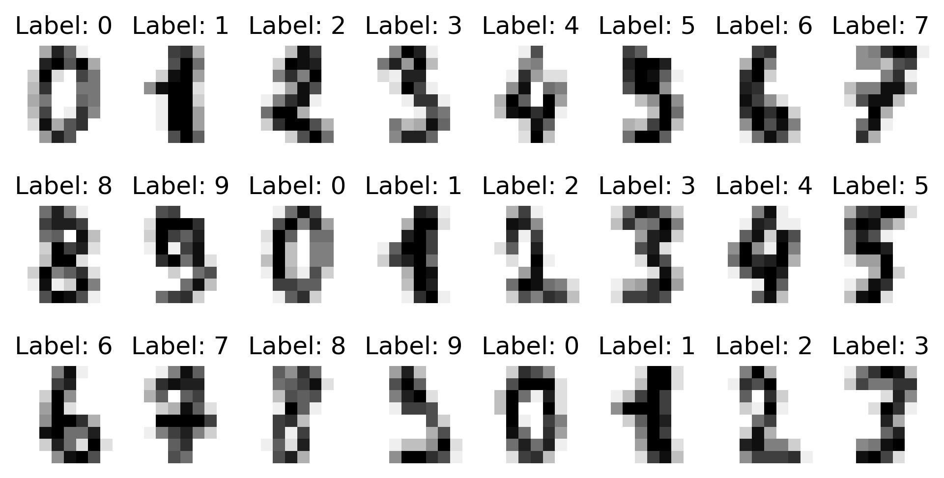
For our first machine learning task, we’ll use the famous MNIST dataset - a collection of handwritten digits that serves as a perfect introduction to image classification. The MNIST dataset has become the “Hello World” of machine learning for good reason:
- Simple to understand (handwritten digits from 0-9)
- Small enough to train quickly
- Complex enough to demonstrate real ML concepts
- Perfect for learning classification basics
Let’s start by loading and exploring this dataset:
# Load dataset
from sklearn import datasets

digits = datasets.load_digits()

# Extract feature matrix X and target vector y
X = digits['data']
y = digits['target']

print(f"Dimension of X: {X.shape}\nDimension of y: {y.shape}")
Dimension of X: (1797, 64)
Dimension of y: (1797,)
Each of our 1,797 samples contains 64 features, representing an 8 x 8 pixel grid of an image. Let’s reshape these features into their original pixel grid format for visualization.
_, axes = plt.subplots(nrows=3, ncols=8, figsize=(8, 4))
for ax, image, label in zip(axes.ravel(), digits.images, digits.target):
    ax.imshow(image, cmap=plt.cm.gray_r, interpolation='nearest')
    ax.set_title("Label: %i" % label)
    ax.set_axis_off()
2. Split data into train and test set
Next, we need to perform a train/test split so that we can validate the final performance of our trained model.
For the train/test split, we will use a 80:20 ratio. Furthermore, we will use the stratify parameter to
ensure that the class distribution in the train and test set is preserved.
from sklearn.model_selection import train_test_split

X_tr, X_te, y_tr, y_te = train_test_split(X, y, test_size=0.2, stratify=y)
3. Train model
For our first classification attempt, we’ll use a RandomForestClassifier. While there are many algorithms to choose from, Random Forests are an excellent starting point because they:
- Handle both numerical and categorical data naturally
- Require minimal preprocessing
- Provide insights into feature importance
- Are relatively robust against overfitting
- Perform well even with default parameters
from sklearn.ensemble import RandomForestClassifier

# Define type of classifier
clf = RandomForestClassifier()

# Train classifier on training data
clf.fit(X_tr, y_tr)

# Evaluate model performance on training and test set
score_tr = clf.score(X_tr, y_tr)
score_te = clf.score(X_te, y_te)

print(
    f"Model accuracy on train data: {score_tr*100:.2f}%\n\
Model accuracy on test data:  {score_te*100:.2f}%"
)
Model accuracy on train data: 100.00%
Model accuracy on test data:  96.67%
The model’s performance metrics reveal several key insights:
- Perfect Training Accuracy (100%): This suggests the model has completely memorized the training data, which could indicate overfitting.
- Strong Test Accuracy (96.67%): Despite potential overfitting, the model generalizes well to unseen data.
- Train-Test Gap (3.33%): The difference between train and test accuracy suggests some overfitting, but it’s within acceptable limits for this task.
- Practical Impact: For digit recognition, 96.67% accuracy means the model would correctly identify about 967 out of 1000 handwritten digits, making it suitable for many real-world applications like postal code reading or form processing.
As you can see, the model performed perfectly on the training set. No wonder, we tested the classifier’s performance on the same data it was trained on. But is there way how we can improve the score on the test data?
Yes there is. But for this we need to fine-tune our random forest classifier. Because as of now we only used the classifier with it’s default parameters.
4. Fine-tune model
To fine-tune our classifier model we need to split our dataset into a third part, the so called validation set. In short, the training set is used to train the parameter of a model, the validation set is used to fine-tune the hyperparameter of a model, and the test set is used to see how well the fine-tuned model generalizes on never before seen data.
A common practice for model validation is k-fold cross-validation. In this approach, the training data is iteratively split into training and validation sets, where each split (or fold) is used once as the validation set.
Now, we also mentioned fine-tuning our model. One way to do this, is to perform a grid search, i.e. running the model with multiple parameter combinations and than deciding which ones work best.
Luckily, scikit-learn provides a neat routine that combines the cross-validation with the grid search, called
GridSearchCV.
So let’s go ahead and set everything up.
from sklearn.model_selection import GridSearchCV

# Define parameter grid
parameters = {'max_depth': [5, 25, 50],  # Controls tree depth - lower values reduce overfitting
             'n_estimators': [1, 10, 50, 200]}  # Number of trees in forest - more trees = better generalization

# Put parameter grid and classifier model into GridSearchCV
grid = GridSearchCV(clf, parameters, cv=5)  # 5-fold cross-validation for robust evaluation

# Train classifier on training data
grid.fit(X_tr, y_tr)

# Evaluate model performance on training and test set
score_tr = grid.score(X_tr, y_tr)
score_te = grid.score(X_te, y_te)

print(
    f"Model accuracy on train data: {score_tr*100:.2f}%\n\
Model accuracy on test data:  {score_te*100:.2f}%"
)
Model accuracy on train data: 100.00%
Model accuracy on test data:  97.22%
Great, our score on the test set has improved. So let’s see which parameter combination seems to be the best.
# Show best random forest classifier
best_rf = grid.best_estimator_
best_rf
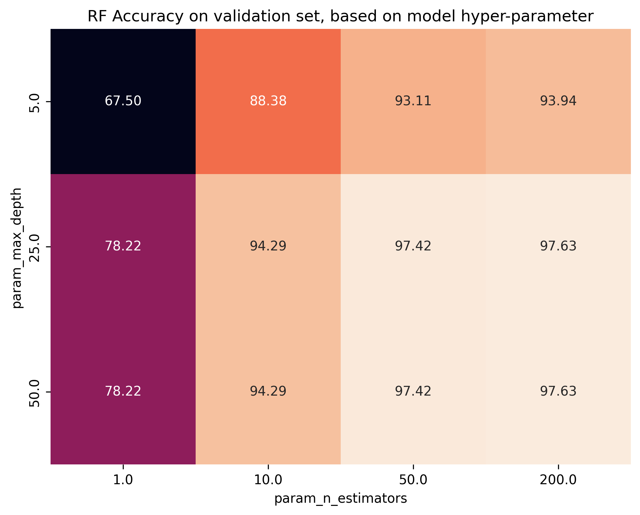
RandomForestClassifier(max_depth=25, n_estimators=200)
Now, to better understand how the different parameters relate to model performance, let’s plot the max_depth
and n_estimators with respect to the accuracy performance on the validation set.
# Put insights from cross-validation grid search into pandas dataframe
df_res = pd.DataFrame(grid.cv_results_)
df_res = df_res.iloc[:, df_res.columns.str.contains('mean_test_score|param_')]
df_res = df_res.astype('float')

# Plot results in table (works only when we investigate two hyper-parameters).
result_table = df_res.pivot(
    index='param_max_depth', columns='param_n_estimators', values='mean_test_score'
)
sns.heatmap(100 * result_table, annot=True, fmt='.2f', square=True, cbar=False)
plt.title("RF Accuracy on validation set, based on model hyper-parameter")
plt.savefig('01_scikit_rf_heatmap.png', bbox_inches='tight', dpi=300)
plt.close()
5. Change model
The great thing about scikit-learn is that the framework is very dynamic. The only thing we need to change to
do the same classification with a Support Vector Machine (SVM) for example, is changing the model and the
parameter grid we want to explore.
# Create support vector classifier object
from sklearn.svm import SVC

clf = SVC(kernel='rbf')

# Define parameter grid
parameters = {
    'C': [0.01, 0.1, 1.0, 10.0, 100.0],  # Regularization parameter - higher values = more complex decision boundary
    'gamma': [0.00001, 0.0001, 0.001, 0.01, 0.1]  # Kernel coefficient - higher values = more influence from nearby points
}
That’s it! The rest can be used as before.
# Put parameter grid and classifier model into GridSearchCV
grid = GridSearchCV(clf, parameters, cv=5)

# Train classifier on training data
grid.fit(X_tr, y_tr)

# Evaluate model performance on training and test set
score_tr = grid.score(X_tr, y_tr)
score_te = grid.score(X_te, y_te)

print(
    f"Model accuracy on train data: {score_tr*100:.2f}%\n\
Model accuracy on test data:  {score_te*100:.2f}%"
)
Model accuracy on train data: 100.00%
Model accuracy on test data:  98.89%
These results show significant improvements:
- Test Accuracy (98.89%): The SVM correctly identifies 989 out of 1000 digits
- Improvement (+2.22%): Compared to Random Forest, SVM reduces errors by about 67%
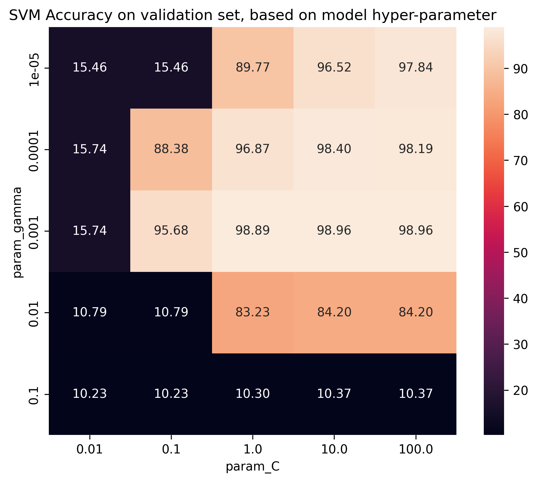
Nice, this is much better. It seems for this particular dataset, with the hyper-parameter’s we explored, SVM is a better model type.
As before, let’s take a look at the model with the best parameters.
# Show best SVM classifier
best_svm = grid.best_estimator_
best_svm
SVC(C=10.0, gamma=0.001)
And once more, how do these two hyper-parameters relate to the performance metric accuracy in the validation
set?
# Put insights from cross-validation grid search into pandas dataframe
df_res = pd.DataFrame(grid.cv_results_)
df_res = df_res.iloc[:, df_res.columns.str.contains('mean_test_score|param_')]
df_res = df_res.astype('float')

# Plot results in table (works only when we investigate two hyper-parameters).
result_table = df_res.pivot(
    index='param_gamma', columns='param_C', values='mean_test_score'
)
sns.heatmap(100 * result_table, annot=True, fmt='.2f', square=True)
plt.title("SVM Accuracy on validation set, based on model hyper-parameter")
plt.savefig('01_scikit_svm_heatmap.png', bbox_inches='tight', dpi=300)
plt.close()
6. Post-model investigation
Last but certainly not least, let’s investigate the prediction quality of our classifier. Two great routines
that you can use for that are scikit-learns
classification_report and
confusion_matrix.
# Predict class predictions on the test set
y_pred = best_svm.predict(X_te)
# Print classification report
from sklearn.metrics import classification_report

print(classification_report(y_te, y_pred))
              precision    recall  f1-score   support
           0       1.00      1.00      1.00        36
           1       1.00      1.00      1.00        36
           2       1.00      1.00      1.00        35
           3       1.00      1.00      1.00        37
           4       1.00      1.00      1.00        36
           5       0.97      0.97      0.97        37
           6       1.00      1.00      1.00        36
           7       0.97      1.00      0.99        36
           8       0.97      1.00      0.99        35
           9       0.97      0.92      0.94        36
    accuracy                           0.99       360
   macro avg       0.99      0.99      0.99       360
weighted avg       0.99      0.99      0.99       360
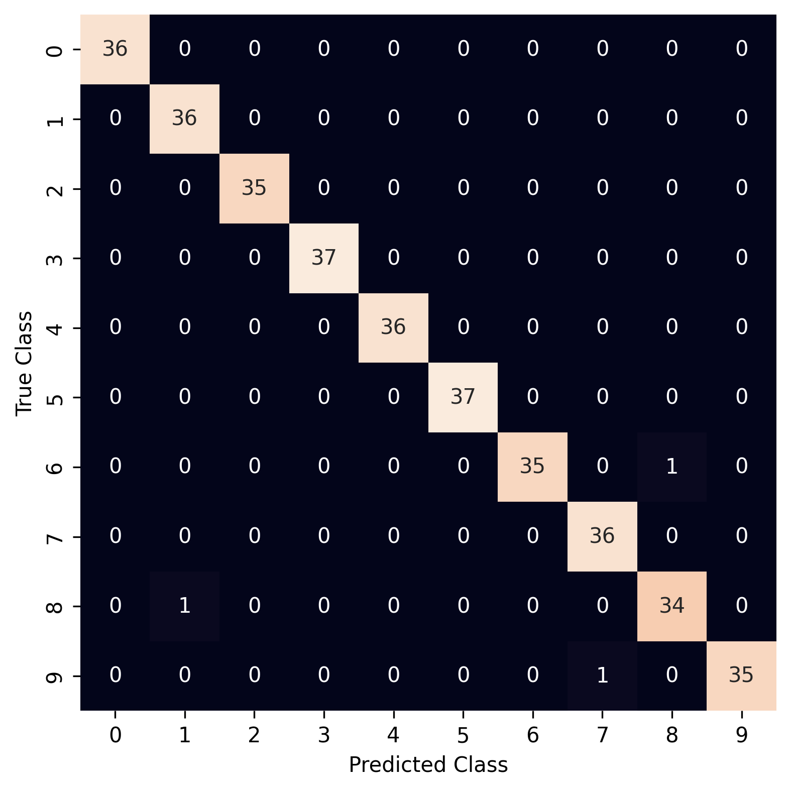
As you can see, while the scores are comparable between classes, some clearly are harder to detect than others. To help better understand which target classes are confused more often than others, we can look at the confusion matrix.
# Compute confusion matrix
from sklearn.metrics import confusion_matrix

cm = confusion_matrix(y_te, y_pred)
sns.heatmap(pd.DataFrame(cm), annot=True, cbar=False, square=True)
plt.xlabel("Predicted Class")
plt.ylabel("True Class")
plt.savefig('01_scikit_confusion_matrix.png', bbox_inches='tight', dpi=300)
plt.close()
7. Additional model and results investigations
Depending on the classifier model you chose, you can investigate many additional things, once your model is trained.
For example, RandomForest model provide a feature_importances_ attribute that allows you to investigate
which of your features is helping the most with the classification task.
# Collect feature importances from RF model
feat_import = best_rf.feature_importances_

# Putting the 64 feature importance values back into 8x8 pixel grid
feature_importance_image = feat_import.reshape(8, 8)

# Visualize the feature importance grid
plt.figure(figsize=(5, 5))
plt.imshow(feature_importance_image)
plt.title("RF Feature Importance")
plt.savefig('01_scikit_feature_importance.png', bbox_inches='tight', dpi=300)
plt.close()
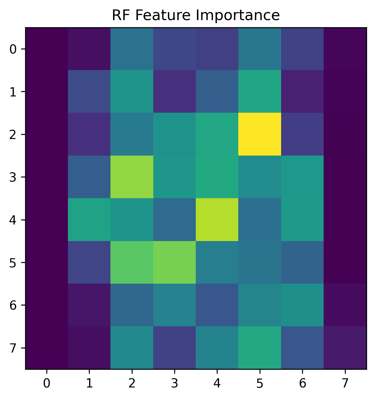
As you can see, feature in the center of the 8x8 grid seem to be more important for the classification task.
Other interesting post-modeling tasks could be the investigation of the prediction probabilities per sample. For example: What do images look like of digits with 100% prediction probability?
# Compute prediction probabilities
y_prob = best_rf.predict_proba(X_te)

# Extract prediction probabilities of target class
target_prob = [e[i] for e, i in zip(y_prob, y_te)]

# Plot images of easiest to predict samples
_, axes = plt.subplots(nrows=3, ncols=20, figsize=(9, 1.5))
for ax, idx in zip(axes.ravel(), np.argsort(target_prob)[::-1]):
    ax.imshow(X_te[idx].reshape(8, 8), cmap=plt.cm.gray_r, interpolation='nearest')
    ax.set_axis_off()
plt.savefig('01_scikit_confident_predictions.png', bbox_inches='tight', dpi=300)
plt.close()

And what about the difficult cases? For which digits does the model strugle the most to get above chance level?
# Plot images of easiest to predict samples
_, axes = plt.subplots(nrows=3, ncols=20, figsize=(9, 1.5))
for ax, idx in zip(axes.ravel(), np.argsort(target_prob)):
    ax.imshow(X_te[idx].reshape(8, 8), cmap=plt.cm.gray_r, interpolation='nearest')
    ax.set_axis_off()
plt.savefig('01_scikit_uncertain_predictions.png', bbox_inches='tight', dpi=300)
plt.close()

Common Pitfalls in Machine Learning Classification
Before wrapping up, let’s discuss some important pitfalls to avoid when working on classification tasks:
Data Leakage: Always split your data before any preprocessing or feature engineering
# Wrong: Preprocessing before split
X_scaled = preprocessing.scale(X)
X_tr, X_te, y_tr, y_te = train_test_split(X_scaled, y)

# Correct: Split first, then preprocess
X_tr, X_te, y_tr, y_te = train_test_split(X, y)
X_tr_scaled = preprocessing.scale(X_tr)
X_te_scaled = preprocessing.scale(X_te)
Class Imbalance: Always check your class distribution
# Show absolute and relative frequencies
class_dist = pd.Series(y).value_counts(normalize=True)
print("Class distribution (%):")
print(class_dist.mul(100).round(2))

# Visualize distribution
class_dist.plot(kind='bar')
plt.title('Class Distribution')
plt.xlabel('Class')
plt.ylabel('Frequency (%)')
Overfitting: Monitor these warning signs - Large gap between training and validation scores - Perfect training accuracy (like we saw with RandomForest) - Poor generalization to new data
# Use cross-validation for robust estimates
from sklearn.model_selection import cross_val_score

scores = cross_val_score(clf, X_tr, y_tr, cv=5)
print(f"CV Scores: {scores}")
print(f"Mean: {scores.mean():.3f} (±{scores.std()*2:.3f})")
Memory Management: For large datasets, consider these approaches
# Use n_jobs parameter for parallel processing
rf = RandomForestClassifier(n_jobs=-1)  # Use all available cores

# Or batch processing with random forests
rf = RandomForestClassifier(max_samples=0.8)  # Use 80% of samples per tree
Feature Scaling: Different algorithms have different scaling requirements
# SVM requires scaling, Random Forests don't
from sklearn.preprocessing import StandardScaler

# For SVM
scaler = StandardScaler()
X_tr_scaled = scaler.fit_transform(X_tr)
X_te_scaled = scaler.transform(X_te)

# Random Forests can handle unscaled data
rf.fit(X_tr, y_tr)  # No scaling needed
Model Selection Bias: Don’t use test set for model selection
# Wrong: Using test set for parameter tuning
for param in parameters:
    clf.set_params(**param)
    score = clf.fit(X_tr, y_tr).score(X_te, y_te)  # Don't do this!

# Correct: Use cross-validation
grid = GridSearchCV(clf, parameters, cv=5)
grid.fit(X_tr, y_tr)
# Only use test set for final evaluation
Model Troubleshooting Tips
# Check for data issues first
print("Missing values:", X.isnull().sum().sum())
print("Infinite values:", np.isinf(X.values).sum())

# Verify predictions are valid
y_pred = clf.predict(X_te)
if len(np.unique(y_pred)) == 1:
    print("Warning: Model predicting single class!")

# Check probability calibration
y_prob = clf.predict_proba(X_te)
if np.any(y_prob > 1.0) or np.any(y_prob < 0.0):
    print("Warning: Invalid probability predictions!")
Common Error Messages and Solutions
-
ValueError: Input contains NaN: Clean your data before training -
MemoryError: Reduce batch size or use data generators
Summary and Next Steps
In this first tutorial, we’ve covered the fundamentals of machine learning with Scikit-learn:
- Loading and visualizing data
- Splitting data into training and test sets
- Training a basic classifier
- Fine-tuning model parameters
- Evaluating model performance
We’ve seen how Scikit-learn’s consistent API makes it easy to experiment with different algorithms and preprocessing techniques. The RandomForest classifier achieved 97.22% accuracy, while the SVM performed even better at 98.89%.
In the next post, we’ll tackle the same MNIST classification problem using TensorFlow, introducing neural networks and deep learning concepts. This will help you understand the differences between classical machine learning approaches and deep learning, and when to use each.
Key takeaways:
- Even simple models can achieve good performance on well-structured problems
- Start with simple models and gradually increase complexity
- Cross-validation is crucial for reliable performance estimation
- Grid search helps find optimal parameters systematically
- Always keep a separate test set for final evaluation
- Look beyond accuracy to understand model performance
In Part 2, we’ll explore how neural networks approach the same problem using TensorFlow, introducing deep learning concepts and comparing the two approaches.