In this third part of our series, we’ll explore more sophisticated machine learning techniques using Scikit-learn. While Parts 1 and 2 focused on classification, we’ll now tackle regression problems and learn how to build complex preprocessing pipelines. We’ll use the California Housing dataset to demonstrate these concepts.

Note: The purpose of this post is to highlight the flexibility and capabilities of scikit-learn’s advanced features. Therefore, this tutorial focuses on introducing you to those advanced routines rather than creating the optimal regression model.

Why Advanced Preprocessing?

Real-world data rarely comes in a clean, ready-to-use format. Data scientists often spend more time preparing data than training models. Common challenges include:

• Missing values that need imputation
• Categorical features requiring encoding
• Features with different scales
• Redundant or irrelevant features
• Non-linear relationships between variables

Scikit-learn provides powerful tools to handle these challenges systematically. Let’s see how to combine them effectively into a preprocessing pipeline that can handle all these issues automatically.

As always, first, let’s import the scientific Python packages we need.

# Standard scientific Python imports
import numpy as np
import matplotlib.pyplot as plt

1. Load Dataset

The California Housing dataset contains information about houses in California districts. It’s a perfect dataset for demonstrating advanced preprocessing because it includes:

• Both numerical and categorical features
• Missing values that need handling
• Features on different scales
• Complex relationships between variables

The dataset itself contains information about the houses, including features like total area, lot shape, neighborhood information, overall quality, year built, etc. And the target feature that we would like to predict is the SalePrice.

Let’s load the data and take a look:

# Load dataset
from sklearn import datasets

housing = datasets.fetch_openml(name='house_prices')

# Extract feature matrix X and target vector y
X = housing['data'].drop(columns='Id')
y = housing['target']

print(f"Dimension of X: {X.shape}\nDimension of y: {y.shape}")

Dimension of X: (1460, 79)
Dimension of y: (1460,)

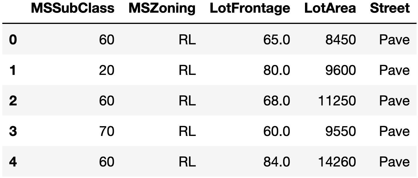
As you can see, we have 1460 samples (houses), each containing 79 features (i.e. characteristics). Let’s examine the first few entries to better understand our data:

# Show first few entries and columns of the dataset
X.iloc[:5, :5]

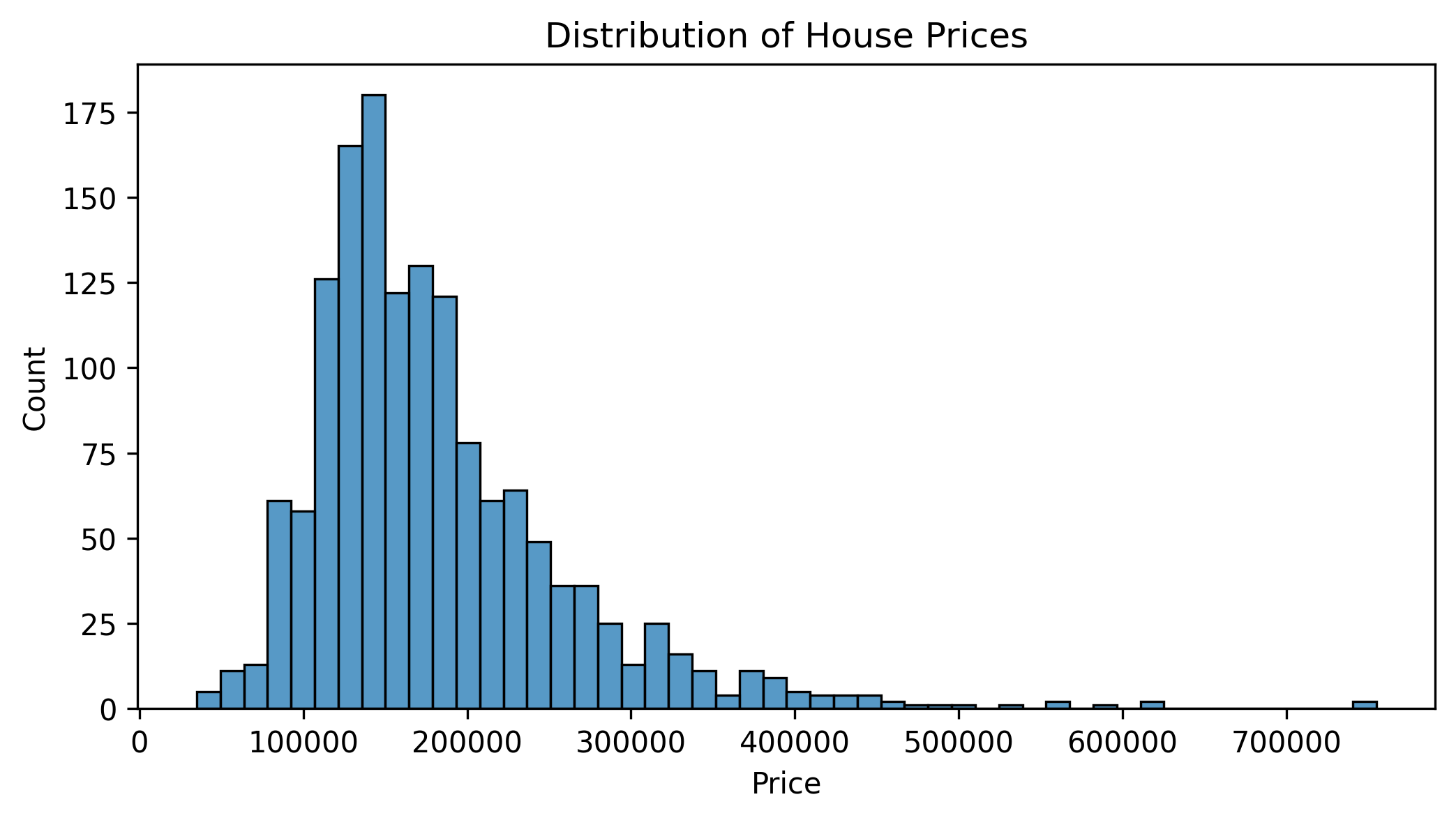
If we look closer at the feature matrix X, we can see that of those 79 features, 36 are of type float and 43 are of type ‘object’ (i.e. categorical features), and that some entries are missing. Plus, the target feature SalePrice has a right skewed value distribution.

Therefore, if possible, our pipeline should be able to handle all of this peculiarities. Even better, let’s try to setup a pipeline that helps us to find the optimal way how to preprocess this dataset.

2. Feature Analysis

Before building our pipeline, let’s understand what we’re working with:

# Quick overview of feature types
print("Feature types:")
print(X.dtypes.value_counts())

# Check for missing values
missing_values = X.isnull().sum()
print("\nFeatures with missing values:")
print(missing_values[missing_values > 0].sort_values(ascending=False))

Feature types:
object     43
int64      33
float64     3
Name: count, dtype: int64

Features with missing values:
PoolQC          1453
MiscFeature     1406
Alley           1369
Fence           1179
FireplaceQu      690
LotFrontage      259
GarageType        81
GarageYrBlt       81
GarageFinish      81
GarageQual        81
GarageCond        81
BsmtExposure      38
BsmtFinType2      38
BsmtFinType1      37
BsmtCond          37
BsmtQual          37
MasVnrArea         8
MasVnrType         8
Electrical         1
dtype: int64

And visualizing the target variable distribution:

# Analyze target variable distribution
import matplotlib.pyplot as plt
import seaborn as sns

plt.figure(figsize=(8, 4))
sns.histplot(y, bins=50)
plt.title("Distribution of House Prices")
plt.xlabel("Price")
plt.show()

This analysis reveals several important preprocessing needs:

1. We have both numerical (float) and categorical (object) features
2. Several features have missing values
3. Our target variable (house prices) shows right skew
4. Features are on very different scales (e.g., year vs. price)

These insights will guide our pipeline design.

3. Split data into train and test set

As always, let’s first go ahead and split the dataset into train and test set.

from sklearn.model_selection import train_test_split

X_tr, X_te, y_tr, y_te = train_test_split(X, y, test_size=0.2)

4. Building the Pipeline

One of Scikit-learn’s most powerful features is its Pipeline API. We’ll create a pipeline that:

1. Handles missing values differently for numerical and categorical features
2. Applies appropriate scaling to numerical features
3. Properly encodes categorical features
4. Optionally reduces dimensionality
5. Fits our chosen regression model

So let’s setup a pipeline that performs these different pre-processing routines: Transformation of categorical data to numerical data, data imputer for missing values, data scaling, potential dimensionality reduction, etc.

Handling categorical data

First, let’s create a small pipeline that takes categorical data, fills missing values with 'missing' and than applies one-hot encoding on these categorical features.

from sklearn.pipeline import Pipeline
from sklearn.impute import SimpleImputer
from sklearn.preprocessing import OneHotEncoder

categorical_preprocessor = Pipeline(
    [
        ('imputer_cat', SimpleImputer(fill_value='missing', strategy='constant')),
        ('onehot', OneHotEncoder(handle_unknown='ignore')),
    ]
)

Handling numerical data

To handle numerical data we will use a slightly more advanced processing pipeline (to showcase some scikit-learn feature, not because it’s the best thing to do). So let’s first fill missing values with e.g. the mean of the feature, potentially apply a polynomial expansion to module non-linear relationships, apply a scaler and then potentially apply dimensionality reduction via PCA and/or by selecting only the “most relevant” features.

from sklearn.decomposition import PCA
from sklearn.feature_selection import SelectKBest
from sklearn.feature_selection import f_regression, mutual_info_regression
from sklearn.pipeline import FeatureUnion

# FeatureUnion performs both processing steps in parallel and combines the features
dim_reduction = FeatureUnion(
    [
        ('pca', PCA()),
        ('feat_selecter', SelectKBest()),
    ]
)

from sklearn.preprocessing import (PolynomialFeatures, StandardScaler,
                                   RobustScaler, PowerTransformer)

# Package all relevant preprocessing routines for numerical data into one pipeline
numeric_preprocessor = Pipeline(
    [
        ('imputer_numeric', SimpleImputer(missing_values=np.nan, strategy='mean')),
        ('polytrans', PolynomialFeatures()),
        ('scaler', StandardScaler()),
        ('dim_reduction', dim_reduction),
    ]
)

Combining preprocessing pipelines

Now that we have a preprocessing pipeline for the categorical and numerical features, let’s combine them into one preprocessing pipeline.

from sklearn.compose import ColumnTransformer

preprocessor = ColumnTransformer(
    [
        ('numerical', numeric_preprocessor, X.select_dtypes('number').columns),
        ('categorical', categorical_preprocessor, X.select_dtypes(exclude='number').columns),
    ],
    remainder='passthrough',
)

Add regression model

After the data is preprocessed we want to hand it over to a regression estimator. For this purpose, let’s chose a ridge regression.

from sklearn.linear_model import Ridge

ridge = Ridge()

pipe = Pipeline(steps=[
    ('preprocessor', preprocessor),
    ('ridge', Ridge())
])

As such, the pipeline would be finished. But because we know that our target feature SalePrice is right skewed, we should ideally apply a log-transformation before fitting the model. Instead of doing this transformation manually (and reverting it at the end), we can also use scikit-learn’s TransformedTargetRegressor to do that on the fly.

from sklearn.compose import TransformedTargetRegressor

regressor = TransformedTargetRegressor(
    regressor=pipe, func=np.log1p, inverse_func=np.expm1
)

5. Parameter grid

Before training our model, we should also define a parameter grid that allows us to fine-tune the processing and model parameters. Given our complex routine, we actually have a lot of parameter that we can play around with.

from sklearn.model_selection import ParameterGrid

# Shorten key identifier by separating common prefix
prefix = 'regressor__preprocessor__'

# Create parametergrid
param_grid = {

    # Explore imputers
    f'{prefix}numerical__imputer_numeric__add_indicator': [True, False],
    f'{prefix}numerical__imputer_numeric__strategy': [
        'mean', 'median', 'most_frequent', 'constant'],
    f'{prefix}categorical__imputer_cat__add_indicator': [True, False],
    f'{prefix}categorical__imputer_cat__strategy': ['most_frequent', 'constant'],

    # Explore numerical preprocessors
    f'{prefix}numerical__polytrans__degree': [1, 2],
    f'{prefix}numerical__polytrans__interaction_only': [False, True],
    f'{prefix}numerical__dim_reduction__pca': ['drop', PCA(0.9), PCA(0.99)],
    f'{prefix}numerical__dim_reduction__feat_selecter__k': [5, 25, 100, 'all'],
    f'{prefix}numerical__dim_reduction__feat_selecter__score_func': [
        f_regression, mutual_info_regression],

    # Explore scalers
    f'{prefix}numerical__scaler': [StandardScaler(), RobustScaler(), PowerTransformer()],

    # Explore regressor
    'regressor__ridge__alpha': np.logspace(-5, 5, 11),
}

print(len(ParameterGrid(param_grid)))

101376

As you can see, we have more than 100’000 different parameter combinations that we could explore. So using a GridSearchCV routine and checking all of them individually would take way too much time. Luckily, scikit-learn also provides a RandomizedSearchCV routine, with which you can randomly explore a few parameter grid combinations.

Furthermore, both GridSearchCV and RandomizedSearchCV routines also allow you to change the performance metric with which the model performs is scored. So let’s take 'neg_mean_absolute_percentage_error' (for more see here).

from sklearn.model_selection import RandomizedSearchCV

random_search = RandomizedSearchCV(
    regressor,
    param_grid,
    n_iter=250,
    refit=True,
    cv=2,
    return_train_score=True,
    n_jobs=-1,
    verbose=1,
    scoring='neg_mean_absolute_percentage_error',
)

6. Train model

Everything is ready, so let’s go ahead and train the model.

res = random_search.fit(X_tr, y_tr)

Fitting 2 folds for each of 250 candidates, totalling 500 fits

7. Performance investigation after RandomizedSearchCV

Once the model has explored a fixed number of grid points, we can go ahead and look at their performance. The easiest is to just put everything into a pandas DataFrame and sort the entries by the best test score.

import pandas as pd

df_res = pd.DataFrame(res.cv_results_)
df_res = df_res.iloc[:, ~df_res.columns.str.contains('time|split[0-9]*|rank|params')]
new_columns = [
    c.split('param_regressor__')[1] if 'param_regressor' in c else c
    for c in df_res.columns
]
new_columns = [
    c.split('preprocessor__')[1] if 'preprocessor__' in c else c for c in new_columns
]
df_res.columns = new_columns
df_res = df_res.sort_values('mean_test_score', ascending=False)
df_res.head(10)

If you explore this table a bit you can better judge which parameter variations in your grid search are actually useful and which ones aren’t. In this example we will not focus on this and directly continue with computing the model performance on the training and test set.

# Evaluate model performance on training and test set
score_tr = -random_search.score(X_tr, y_tr)
score_te = -random_search.score(X_te, y_te)

print(
    f"Prediction accuracy on train data: {score_tr*100:.2f}%\n\
Prediction accuracy on test data:  {score_te*100:.2f}%"
)

Prediction accuracy on train data: 7.10%
Prediction accuracy on test data:  8.38%

Great, the score seems reasonably good! But now that we know better which preprocessing routine seems to be the best (thanks to RandomizedSearchCV), let’s go ahead and further fine-tune the ridge model.

8. Fine tune best preprocessing pipeline

To further fine tune the best preprocessing pipeline, we can just load the ‘best estimator’ from the RandomizedSearchCV exploration and specify a new parameter grid that we want to explore - this time with the GridSearchCV routine (so that we look at all grid points).

# Select best estimator
best_estimator = random_search.best_estimator_

# Specify new parameter grid to explore
param_grid = {'regressor__ridge__alpha': np.logspace(-5, 5, 51)}

To showcase one more additional thing, let’s go ahead and use a nested cross-validation routine to improve the generalization power of our model. In other words, in contrast to the previous approach where we separated the test from the train set only once, we will now also apply a cross validation approach on this split as well. Together with the cross validation in the grid search, we therefore use cross validation twice, hence the name “nested”.

# Establish the two cross validations
from sklearn.model_selection import KFold

inner_cv = KFold(n_splits=3, shuffle=True)
outer_cv = KFold(n_splits=3, shuffle=True)

And now, let’s combine all of this with and run the model.

from sklearn.model_selection import GridSearchCV, cross_validate

# Create grid search object with parameter grid and inner cross validation
grid_search = GridSearchCV(
    best_estimator,
    param_grid,
    refit=True,
    cv=inner_cv,
    n_jobs=-1,
    scoring='neg_mean_absolute_percentage_error',
)

# Train model with outer cross validation (and return estimators for post-model investigation)
cv_results = cross_validate(
    grid_search,
    X=X,
    y=y,
    cv=outer_cv,
    n_jobs=1,
    return_estimator=True,
    return_train_score=True,
)

Once the model has finished training, we can extract the different scores from the most outer loop and print their average score, as well as the standard deviation over the folds. Plus, the same thing can also be done for the most optimal ridge model parameter ‘alpha’. These information can give us some insights about the model generalization.

df_nested = pd.DataFrame(cv_results)
cv_train_scores = -df_nested['train_score']
cv_test_scores = -df_nested['test_score']
cv_alphas = [c.best_params_['regressor__ridge__alpha'] for c in df_nested['estimator']]
print(
    "Generalization score with hyperparameters tuning:\n"
    f"  Train Score:    {cv_train_scores.mean()*100:.1f}% +/- {cv_train_scores.std()*100:.1f}%\n"
    f"  Test Score:     {cv_test_scores.mean()*100:.1f}% +/- {cv_test_scores.std()*100:.1f}%\n"
    f"  Optimal Alpha: {np.mean(cv_alphas):.1f} +/- {np.std(cv_alphas):.1f}\n"
)

Generalization score with hyperparameters tuning:
  Train Score:    7.6% +/- 0.9%
  Test Score:     9.0% +/- 0.2%
  Optimal Alpha: 29.6 +/- 23.8

9. Feature importance investigation with permutation testing

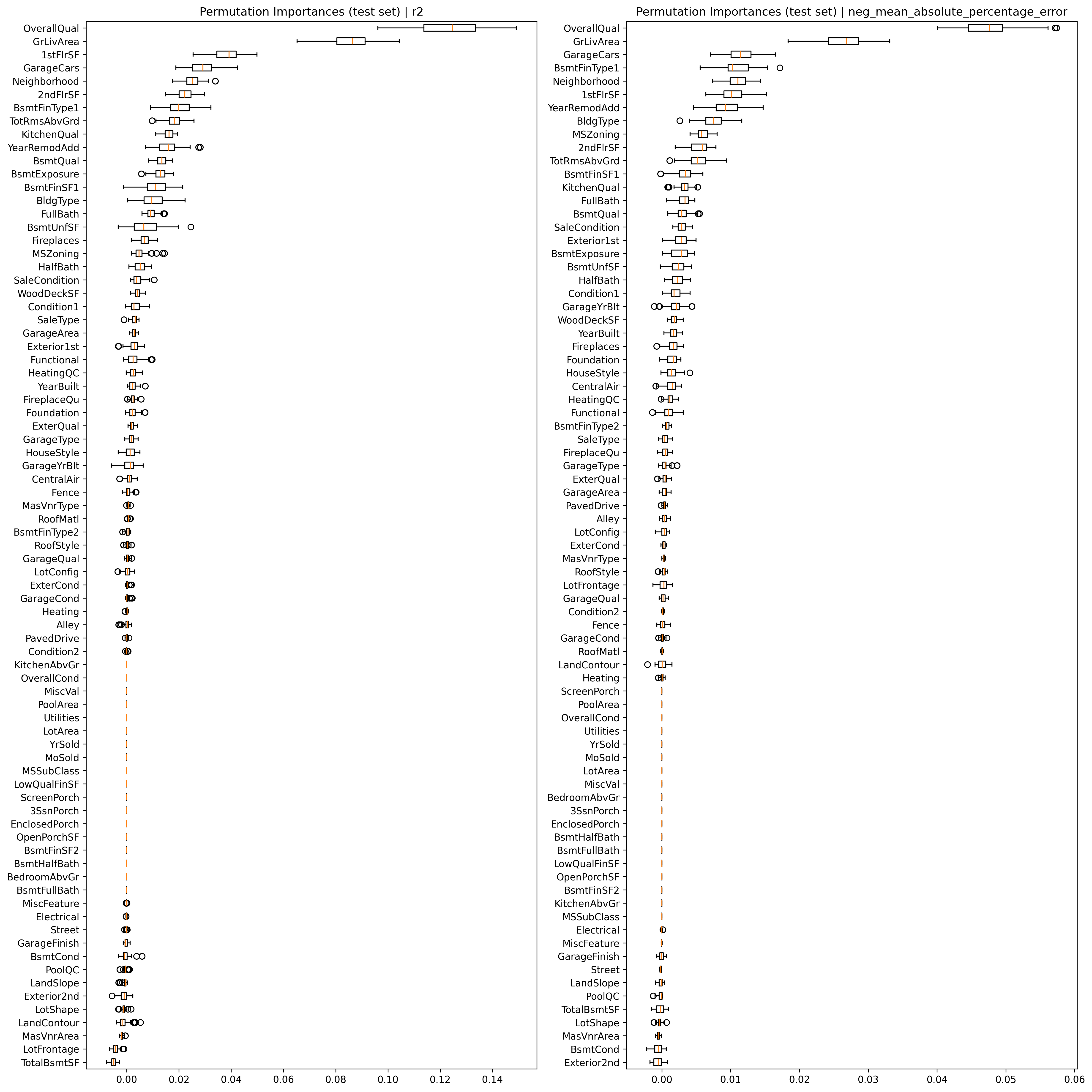
Some model provide some insights about feature importance (i.e. which features the model uses most for the prediction). However, this is sometimes prone to multiple issues. A better approach is to use a permutation approach. This approach performs the same model fitting (in this case based on the best model with the best hyper parameters) but during each iteration randomly shuffles a given feature and investigates how this perturbates the final score.

# Select the best estimator with the best hyper parameter
final_estimator = grid_search.set_params(
    estimator__regressor__ridge__alpha=np.mean(cv_alphas)
)

# Fit this estimator to the initial training set
_ = final_estimator.fit(X_tr, y_tr)

Now that the model is ready and trained, we can go ahead and perform the feature importance investigation via permutation testing. To showcase one additional feature, let’s actually perform this routine twice, once while focusing on the r2 of the model, and once while focusing on the neg_mean_absolute_percentage_error.

from sklearn.inspection import permutation_importance

scoring = ['r2', 'neg_mean_absolute_percentage_error']
result = permutation_importance(
    final_estimator,
    X_te,
    y_te,
    n_repeats=50,
    random_state=0,
    n_jobs=-1,
    scoring=scoring,
)

Once everything is computed, we can go ahead and plot the feature importance for each feature, separated by the two different scoring metrics.

fig, axs = plt.subplots(1, 2, figsize=(16, 16))
for i, s in enumerate(scoring):

    sorted_idx = result[s].importances_mean.argsort()

    axs[i].boxplot(
        result[s].importances[sorted_idx].T, vert=False, labels=X_te.columns[sorted_idx]
    )
    axs[i].set_title("Permutation Importances (test set) | %s" % s)
fig.tight_layout()
plt.show()

Summary and Next Steps

In this tutorial, we’ve covered advanced scikit-learn concepts:

• Building complex preprocessing pipelines
• Handling mixed data types
• Feature selection and engineering automatically
• Implementing grid search with cross-validation
• Model comparison and evaluation
• Analyzing feature importance

Key takeaways:

1. Preprocessing pipelines make complex workflows manageable
2. Grid search helps find optimal parameters systematically
3. Feature selection can improve model performance
4. Understanding feature importance aids model interpretation
5. Cross-validation provides robust performance estimates

In Part 4, we’ll explore advanced neural network architectures with TensorFlow, building on both the neural network concepts from Part 2 and the preprocessing techniques we’ve learned here.

← Back to Part 2 or Continue to Part 4 →