How to use fMRI multi-slice acquisition correctly
fMRI multi-slice acquisition
Up until a few years back, functional MRI images of a human’s brain had to be recorded volume by volume, slice by slice. Meaning, that for each time-point, i.e. each sampling point, in an fMRI dataset, the MRI scanner had to first record ~40 consecutive slices (covering the full brain), one after the other. So, if one slice takes 50m to record, that means one full brain volume will take 2000ms to record. Or in other words, the fMRI signal was recorded with a sampling rate of 2 seconds.
While this technological achievement provided already enough detail to establish many great neuroimaging studies, it nonetheless was one of the reasons why fMRI data was considered a ‘rather slow’ neuroimaging method. Luckily, new advancements in the field, allowed the acceleration of the data acquisition by establish a method where multiple slices can be acquired in parallel. So, if we acquired 2 slices in parallel, the acceleration factor became 2, and if it’s 4 slices, the acceleration factor is 4. This acceleration factor also directly effects the sampling rate, which means that a temporal resolution of 1 second (using acceleration of 2) or 500ms (using acceleration of 4) became possible.
For a visual comparison between different approaches, see the following gif (note, top left is the acquisition without any acceleration).
I’ve created this nice-looking gif for my PhD defense, but thought that others might also be interested in seeing the striking difference in temporal resolution as well. I therefore shared my gif via twitter, and to my delight, the tweet was met with lots of shared excitement and fascination:
Ever wondered what the difference between single- and multi-slice acquisition would look like? Here's a visualization of a 🧠 volume with an acceleration factor of 1, 2, 3 or 4, leading to a TR of 2s, 1s, 0.66s and 0.5s. pic.twitter.com/cLMHykZIMi
— Michael Notter (@miyka_el) June 23, 2021
The drawback
The usage of such multi-slice approaches obviously also comes with drawbacks. If the acceleration factor is too high, the data quality (or signal-to-noise ratio) decreases too much. But if it’s done just right, sub-second recording of fMRI becomes possible.
However, this is not the only drawback with regards to improved sampling rate. For my PhD thesis, I recorded a huge 17 subject big fMRI dataset with six 5min long functional recordings, at a temporal resolution of 600ms. And while preprocessing my data as usual, I suddenly stumbled over something rather unusual.
The following three figures on the left show the recorded average signal activation throughout the brain (i.e. in the ‘total volume’ = TV), plus two of the six estimated motion parameters (rotation around x-axis = Rotation01; translation in z-direction = Translation03). And on the right, you can see the corresponding frequency power spectrum.
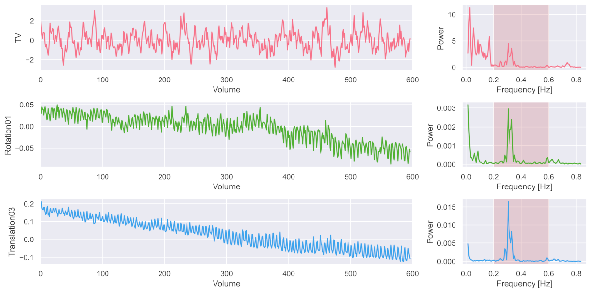
What is striking is that all of these three methods have a particular oscillation in the higher frequency of ~0.3 Hz. Which perfectly corresponds to the respiratory frequency (i.e. breathing) that people usually have in the fMRI scanner.
In other words, due to improved sampling rate through multi-slice acquisition, fMRI recording now was capable of recording nuance components such as respiratory or cardiac (at 1 to 1.7 Hz) signal (for more see Viessman et al., 2018).
The problem
While this might be nice to have, problems actually start arising when we preprocess such “temporal high-res” data as we normally would (see Lindquist et al., 2019). If during the preprocessing we apply standard motion correction and potential temporal filtering with a low-pass filter, we might reintroduce previously cleaned noise components.
To counter this issue, I developed a method that allows the orthogonal cleaning of such fMRI data with the effect of properly removing respiratory (and cardiac) artefacts. So let’s take another look at the three signal curves we had from before after we preprocessed the data with my new approach.
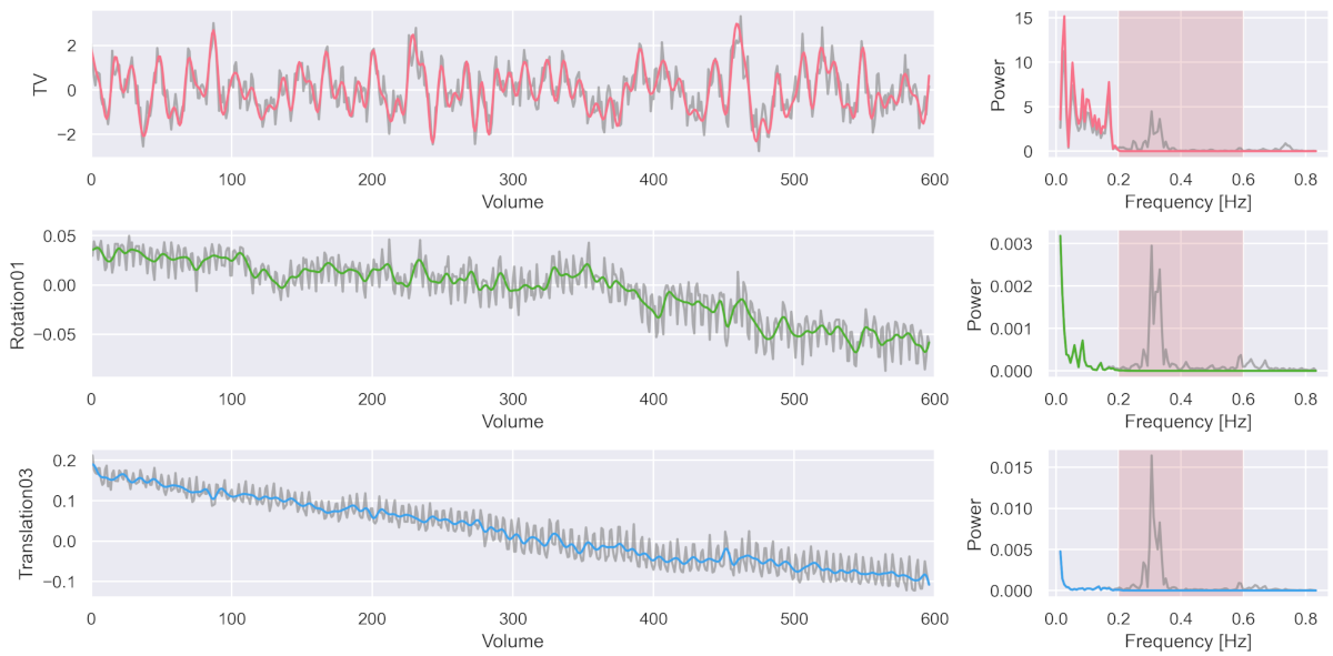
The colored signal shows the cleaned signal, while the gray signal was the one from before the cleaning. As you can see, the noise component was nicely removed.
The good
While this might be a nice thing to do, the actual advantage of doing it the right way becomes more obvious once we look at the output of a standard fMRI analysis.
The following illustration shows a single subject’s statistical map of the brain activation differences during audio-visual versus audio only stimulation, using 5 different analysis methods. Panel A) shows my newly developed approach using a temporal low-pass filter at 0.2Hz, panel B) shows the same approach without the temporal low-pass filter and panel C) to E) show the comparable state of the art neuroimaging toolboxes fMRIPrep, FSL and SPM.
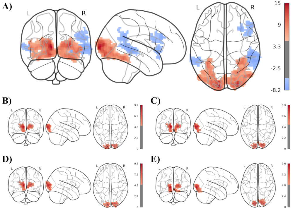
What is clearly visible is that my approach in panel A), using an appropriate low-pass filter with orthogonal preprocessing leads to much stronger statistical results, even just in the single subject (i.e 1st-level) analysis.
fMRIflows
I packaged this improved fMRI preprocessing technique and much more into my neuroimaging toolbox fMRIflows.

For more about fMRIflows and this approach, feel free to take a look at the corresponding scientific paper or an explanation of the even brother implications in my PhD thesis.