Iterables
Some steps in a neuroimaging analysis are repetitive. Running the same preprocessing on multiple subjects or doing statistical inference on multiple files. To prevent the creation of multiple individual scripts, Nipype has as execution plugin for Workflow, called iterables.

If you are interested in more advanced procedures, such as synchronizing multiple iterables or using conditional iterables, check out the synchronizeand intersource section in the JoinNode notebook.
Realistic example
Let's assume we have a workflow with two nodes, node (A) does simple skull stripping, and is followed by a node (B) that does isometric smoothing. Now, let's say, that we are curious about the effect of different smoothing kernels. Therefore, we want to run the smoothing node with FWHM set to 2mm, 8mm, and 16mm.
from nipype import Node, Workflow
from nipype.interfaces.fsl import BET, IsotropicSmooth

# Initiate a skull stripping Node with BET
skullstrip = Node(BET(mask=True,
                      in_file='/data/ds000114/sub-01/ses-test/anat/sub-01_ses-test_T1w.nii.gz'),
                  name="skullstrip")
Create a smoothing Node with IsotropicSmooth
isosmooth = Node(IsotropicSmooth(), name='iso_smooth')
Now, to use iterables and therefore smooth with different fwhm is as simple as that:
isosmooth.iterables = ("fwhm", [4, 8, 16])
And to wrap it up. We need to create a workflow, connect the nodes and finally, can run the workflow in parallel.
# Create the workflow
wf = Workflow(name="smoothflow")
wf.base_dir = "/output"
wf.connect(skullstrip, 'out_file', isosmooth, 'in_file')

# Run it in parallel (one core for each smoothing kernel)
wf.run('MultiProc', plugin_args={'n_procs': 3})
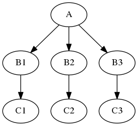
Note, that iterables is set on a specific node (isosmooth in this case), but Workflow is needed to expend the graph to three subgraphs with three different versions of the isosmooth node.
If we visualize the graph with exec, we can see where the parallelization actually takes place.
# Visualize the detailed graph
from IPython.display import Image
wf.write_graph(graph2use='exec', format='png', simple_form=True)
Image(filename='/output/smoothflow/graph_detailed.png')
If you look at the structure in the workflow directory, you can also see, that for each smoothing, a specific folder was created, i.e. _fwhm_16.
!tree /output/smoothflow -I '*txt|*pklz|report*|*.json|*js|*.dot|*.html'
Now, let's visualize the results!
from nilearn import plotting
%matplotlib inline
plotting.plot_anat(
    '/data/ds000114/sub-01/ses-test/anat/sub-01_ses-test_T1w.nii.gz', title='original',
    display_mode='z', dim=-1, cut_coords=(-50, -35, -20, -5), annotate=False);
plotting.plot_anat(
    '/output/smoothflow/skullstrip/sub-01_ses-test_T1w_brain.nii.gz', title='skullstripped',
    display_mode='z', dim=-1, cut_coords=(-50, -35, -20, -5), annotate=False);
plotting.plot_anat(
    '/output/smoothflow/_fwhm_4/iso_smooth/sub-01_ses-test_T1w_brain_smooth.nii.gz', title='FWHM=4',
    display_mode='z', dim=-0.5, cut_coords=(-50, -35, -20, -5), annotate=False);
plotting.plot_anat(
    '/output/smoothflow/_fwhm_8/iso_smooth/sub-01_ses-test_T1w_brain_smooth.nii.gz', title='FWHM=8',
    display_mode='z', dim=-0.5, cut_coords=(-50, -35, -20, -5), annotate=False);
plotting.plot_anat(
    '/output/smoothflow/_fwhm_16/iso_smooth/sub-01_ses-test_T1w_brain_smooth.nii.gz', title='FWHM=16',
    display_mode='z', dim=-0.5, cut_coords=(-50, -35, -20, -5), annotate=False);
IdentityInterface (special use case of iterables)
We often want to start our worflow from creating subgraphs, e.g. for running preprocessing for all subjects. We can easily do it with setting iterables on the IdentityInterface. The IdentityInterface interface allows you to create Nodes that does simple identity mapping, i.e. Nodes that only work on parameters/strings.
For example, you want to start your workflow by collecting anatomical files for 5 subjects.
# First, let's specify the list of subjects
subject_list = ['01', '02', '03', '04', '05']
Now, we can create the IdentityInterface Node
from nipype import IdentityInterface
infosource = Node(IdentityInterface(fields=['subject_id']),
                  name="infosource")
infosource.iterables = [('subject_id', subject_list)]
That's it. Now, we can connect the output fields of this infosource node to SelectFiles and DataSink nodes.
from os.path import join as opj
from nipype.interfaces.io import SelectFiles, DataSink

anat_file = opj('sub-{subject_id}', 'ses-test', 'anat', 'sub-{subject_id}_ses-test_T1w.nii.gz')

templates = {'anat': anat_file}

selectfiles = Node(SelectFiles(templates,
                               base_directory='/data/ds000114'),
                   name="selectfiles")

# Datasink - creates output folder for important outputs
datasink = Node(DataSink(base_directory="/output",
                         container="datasink"),
                name="datasink")

wf_sub = Workflow(name="choosing_subjects")
wf_sub.connect(infosource, "subject_id", selectfiles, "subject_id")
wf_sub.connect(selectfiles, "anat", datasink, "anat_files")
wf_sub.run()
Now we can check that five anatomicl images are in anat_files directory:
! ls -lh /output/datasink/anat_files/
This was just a simple example of using IdentityInterface, but a complete example of preprocessing workflow you can find in Preprocessing Example).
Exercise 1
Create a workflow to calculate various powers of 2 using two nodes, one for IdentityInterface with iterables, and one for Function interface to calculate the power of 2.
# write your solution here
# lets start from the Identity node
from nipype import Function, Node, Workflow
from nipype.interfaces.utility import IdentityInterface

iden = Node(IdentityInterface(fields=['number']), name="identity")
iden.iterables = [("number", range(8))]
# the second node should use the Function interface
def power_of_two(n):
    return 2**n

# Create Node
power = Node(Function(input_names=["n"],
                      output_names=["pow"],
                      function=power_of_two),
              name='power')
#and now the workflow
wf_ex1 = Workflow(name="exercise1")
wf_ex1.connect(iden, "number", power, "n")
res_ex1 = wf_ex1.run()

# we can print the results
for i in range(8):
    print(list(res_ex1.nodes())[i].result.outputs)