![]()
Table of Contents
- How To Build A Pipeline
![]()
Important
This guide hasn’t been updated since January 2017 and is based on an older version of Nipype. The code in this guide is not tested against newer Nipype versions and might not work anymore. For a newer, more up to date and better introduction to Nipype, please check out the the Nipype Tutorial.
So, you’ve installed Nipype on your system? And you’ve prepared your dataset for the analysis? This means that you are ready to start this tutorial.
The following section is a general step by step introduction on how to build a pipeline. It will first introduce you to the building blocks of any pipeline, then show you an example of how a basic pipeline is implemented, how to read the output, and most importantly how to tackle problems. At the end you should understand what a pipeline is, how the key parts interact with each other, and how to solve certain issues. In short, you should be able to build any kind of neuroimaging pipeline that you like. So let’s get started!
Before we get into the details, we should explain that Nipype pipelines, or workflows, the terms are synonomous, are made up of nodes and workflows. We will generally use ‘workflow’ when referring to section in a script and ‘pipeline’ to refer to the whole construction that is actually run.
Briefly, you can think of a node as a unit of processing; for example, a node will run the program to smooth data. Nodes are most often associated with analytic interfaces to, say, FSL, SPM, or AFNI, but they can also be a function to gather the list of image files to be used. Each node is a step in the pipeline.
A workflow is a collection of nodes and the rules that connect the nodes to each other. Typically, the output of one node is attached to the input of another node in a workflow. Workflows can also connect other workflows, so you might have a preprocessing workflow, a first-level workflow, a second-level workflow, etc., perhaps with other nodes in between.
Refer back to the diagram of a Nipype workflow on the Nipype and Neuroimaging page. There, the purple box represents an fMRI workflow, and it contains a Preprocessing workflow (the pink box), a functional analysis workflow (the light green box), which in turn contains a 1st level analysis workflow and a 2nd level analysis workflow.
The following example pipeline is based on the preprocessing steps of a functional MRI study. We can usefully categorize in a general way the sections of a pipeline script based on what function each section plays. The sections are common to virtually all pipelines, even though the specific nodes may vary. For that reason, it’s important to understand the sections, how they relate to each other, and what their role in the overall pipeline is.
Import modules: The first step in any script is to import necessary functions and modules needed for data manipulation and analysis.
Specify variables: The second step is to define all the variables you will use throughout the script. This is best done in just one place, and I recommended you to do this as the second step, right after module importation.
Specify Nodes: The third step is to define the nodes you will use in
your pipeline. Each node will assign a name to its inputs and to its outputs, and any parameters that are needed for the node to do its job will be defined or assigned to an argument here.
Specify Workflows & Connect Nodes: The fourth step is to define at least
one workflow, though possibly more. The workflows order the nodes and connect them to each other to create the processing stream, insuring that the nodes are executed in the proper order and produce the necessary input for the next node in the workflow.
Input & Output Stream: The fifth step is to specify the structure of
your data folders. The purpose of the input stream is to specify in which folders and under what names the input data is stored. The output stream specifies in which folders output data is stored, which may well be different from where the input data is stored.
Run Workflow: The final step is to actually run the outermost
workflow to do the work and make you famous!
So, make yourself ready, start an IPython environment (type ipython into
the terminal) and have fun creating this example workflow.
The first thing you should do in any script is to import the modules you want to use in your script. In our case, most modules are actually interfaces to other software packages (e.g. FSL, FreeSurfer or SPM) and can be found in the nipype module.
If you want to import a module as a whole use the command structure import <module> as <name>. For example:
# Import the SPM interface under the name spm
import nipype.interfaces.spm as spm
If you only want to import a certain function of a module use the command structure from <module> import <function>. For example:
# Import the function 'maths' from the FSL interface
from nipype.interfaces.fsl import maths
And if you want to import multiple functions or classes from a module use the following structure:
# Import nipype Workflow, Node and MapNode objects
from nipype.pipeline.engine import Workflow, Node, MapNode
There are always variables that change between analysis or that are specific for a certain computer structure. That’s why it is important to keep them all together and at one place. This allows you to be fast, flexible and to keep the changes in your script just to this section.
So which variables should you declare in this section? All of them! Every variable that you change more than once between analysis should be specified here.
For example:
1 2 3 4 5 6 7 8 9 10 11 12 13 14 | # What is the location of your experiment folder
experiment_dir = '~/nipype_tutorial'
# What are the names of your subjects
subjects = ['sub001','sub002','sub003']
# What is the name of your working directory and output folder
output_dir = 'output_firstSteps'
working_dir = 'workingdir_firstSteps'
# What are experiment specific parameters
number_of_slices = 40
time_repetition = 2.0
fwhm = 8
|
It is impossible to build a pipeline without any scaffold or objects to build with. Therefore, we first have to create those scaffolds (i.e. workflows) and objects (i.e. nodes or other workflows).
A node is an object that represents a certain interface function, for example SPM’s Realign method. Every node has always at least one input and one output field. The existent of those fields allow Nipype to connect different nodes to each other and therefore guide the stream of input and output between the nodes.
Nipype provides so many different interfaces with each having a lot of different functions (for a list of all interfaces go here. So how do you know which input and output field a given node has? Don’t worry. There’s an easy way how you can figure out which input fields are mandatory or optional and which output fields you can use.
Let’s assume that we want to know more about FSL’s function SmoothEstimate. First, make sure that you’ve imported the fsl module with the following python command import nipype.interfaces.fsl as fsl.
Now that we have access to FSL, we simply can run fsl.SmoothEstimate.help(). This will give us the following output:
1 2 3 4 5 6 7 8 9 10 11 12 13 14 15 16 17 18 19 20 21 22 23 24 25 26 27 28 29 30 31 32 33 34 35 36 37 38 39 40 41 42 43 44 45 46 47 48 49 50 51 52 53 54 | Wraps command **smoothest**
Estimates the smoothness of an image
Examples
--------
>>> est = SmoothEstimate()
>>> est.inputs.zstat_file = 'zstat1.nii.gz'
>>> est.inputs.mask_file = 'mask.nii'
>>> est.cmdline
'smoothest --mask=mask.nii --zstat=zstat1.nii.gz'
Inputs::
[Mandatory]
dof: (an integer)
number of degrees of freedom
flag: --dof=%d
mutually_exclusive: zstat_file
mask_file: (an existing file name)
brain mask volume
flag: --mask=%s
[Optional]
args: (a string)
Additional parameters to the command
flag: %s
environ: (a dictionary with keys which are a value of type 'str' and
with values which are a value of type 'str', nipype default value: {})
Environment variables
ignore_exception: (a boolean, nipype default value: False)
Print an error message instead of throwing an exception in case the
interface fails to run
output_type: ('NIFTI_PAIR' or 'NIFTI_PAIR_GZ' or 'NIFTI_GZ' or
'NIFTI')
FSL output type
residual_fit_file: (an existing file name)
residual-fit image file
flag: --res=%s
requires: dof
zstat_file: (an existing file name)
zstat image file
flag: --zstat=%s
mutually_exclusive: dof
Outputs::
dlh: (a float)
smoothness estimate sqrt(det(Lambda))
resels: (a float)
number of resels
volume: (an integer)
number of voxels in mask
|
The first few lines (line 1-3) give as a short explanation of the function, followed by a short example on how to implement the function (line 5-12). After the example come information about Inputs (line 14-45) and Outputs (line 47-54). There are always some inputs that are mandatory and some that are optional. Which is not the case for outputs, as they are always optional. It’s important to note that some of the inputs are mutually exclusive (see line 19), which means that if one input is specified, another one can’t be set and will result in an error if it is defined nonetheless.
Important
If you only want to see the example part of the information view, without the details about the input and output fields, use the command fsl.SmoothEstimate?.
If you want to find the location of the actual Nipype script that serves as an interface to the external software package, use also the command fsl.SmoothEstimate? and check out the 3rd line, called File:.
Note
If you want to brows through the different functions, or just want to view the help information in a nicer way, go to the official homepage and either navigate to Interfaces and Algorithms or Documentation.
As you’ve might seen in the example above (line 32), some input fields have Nipype specific default values. To figure out which default values are used for which functions, use the method input_spec().
For example, if you want to know that the default values for SPM’s Threshold function are, use the following command:
1 2 | import nipype.interfaces.spm as spm
spm.Threshold.input_spec()
|
This will give you the following output:
1 2 3 4 5 6 7 8 9 10 11 12 13 14 15 16 | contrast_index = <undefined>
extent_fdr_p_threshold = 0.05
extent_threshold = 0
force_activation = False
height_threshold = 0.05
height_threshold_type = p-value
ignore_exception = False
matlab_cmd = <undefined>
mfile = True
paths = <undefined>
spm_mat_file = <undefined>
stat_image = <undefined>
use_fwe_correction = True
use_mcr = <undefined>
use_topo_fdr = True
use_v8struct = True
|
Nodes are most of the time used inside a pipeline. But it is also possible to use one just by itself. Such a “stand-alone” node is often times very convenient when you run a python script and want to use just one function of a given dependency package, e.g. FSL, and are not really interested in creating an elaborate workflow.
Such a “stand-alone” node is also a good opportunity to introduce the implementation of nodes. Because there are many ways how you can create a node. Let’s assume that you want to create a single node that runs FSL’s Brain Extraction Tool function BET on the anatomical scan of our tutorial subject sub001. This can be achieved in the following three ways:
1 2 3 4 5 6 7 8 9 10 11 12 13 14 15 16 17 18 | # First, make sure to import the FSL interface
import nipype.interfaces.fsl as fsl
# Method 1: specify parameters during node creation
mybet = fsl.BET(in_file='~/nipype_tutorial/data/sub001/struct.nii.gz',
out_file='~/nipype_tutorial/data/sub001/struct_bet.nii.gz')
mybet.run()
# Method 2: specify parameters after node creation
mybet = fsl.BET()
mybet.inputs.in_file = '~/nipype_tutorial/data/sub001/struct.nii.gz'
mybet.inputs.out_file = '~/nipype_tutorial/data/sub001/struct_bet.nii.gz'
mybet.run()
# Method 3: specify parameters when the node is executed
mybet = fsl.BET()
mybet.run(in_file='~/nipype_tutorial/data/sub001/struct.nii.gz',
out_file='~/nipype_tutorial/data/sub001/struct_bet.nii.gz')
|
Hint
To check the result of this execution, run the following command in your terminal:
freeview -v ~/nipype_tutorial/data/sub001/struct.nii.gz \
            ~/nipype_tutorial/data/sub001/struct_bet.nii.gz:colormap=jet
Most of the times when you create a node you want to use it later on in a workflow. The creation of such a “workflow” node is only partly different from the creation of “stand-alone” nodes. The implementation of a “workflow” node has always the following structure:
nodename = Node(interface_function(), name='label')
nodename: This is the name of the object that will be created.
Node: This is the type of the object that will be created. In this case it is a Node. It can also be defined as a MapNode or a Workflow.
interface_function: This is the name of the function this node should represent. Most of the times this function name is preceded by an interface name, e.g. fsl.BET.
label: This is the name, that this node uses to create its working directory or to label itself in the visualized graph.
For example: If you want to create a node called realign that runs SPM’s Realign function on a functional data func.nii, use the following code:
1 2 3 4 5 6 7 8 9 10 11 12 13 14 15 16 17 | # Make sure to import required modules
import nipype.interfaces.spm as spm # import spm
import nipype.pipeline.engine as pe # import pypeline engine
# Create a realign node - Method 1: Specify inputs during node creation
realign = pe.Node(spm.Realign(in_files='~/nipype_tutorial/data/sub001/func.nii'),
name='realignnode')
# Create a realign node - Method 2: Specify inputs after node creation
realign = pe.Node(spm.Realign(), name='realignnode')
realign.inputs.in_files='~/nipype_tutorial/data/sub001/func.nii'
# Specify the working directory of this node (only needed for this specific example)
realign.base_dir = '~/nipype_tutorial/tmp'
# Execute the node
realign.run()
|
Note
This will create a working directory at ~/nipype_tutorial/tmp, containing one folder called realignnode containing all temporary and final output files of SPM’s realign function.
If you’re curious what the realign function just calculated, use the following python commands to plot the estimated translation and rotation parameters of the functional scan func.nii:
1 2 3 4 5 6 7 8 9 10 11 12 13 14 15 16 17 | # Import necessary modules
import numpy
import matplotlib.pyplot as plt
# Load the estimated parameters
movement=numpy.loadtxt('~/nipype_tutorial/tmp/realignnode/rp_func.txt')
# Create the plots with matplotlib
plt.subplot(211)
plt.title('translation')
plt.plot(movement[:,:3])
plt.subplot(212)
plt.title('rotation')
plt.plot(movement[:,3:])
plt.show()
|
Iterables are a special kind of input fields and any input field of any Node can be turned into an Iterable. Iterables are very important for the repeated execution of a workflow with slightly changed parameters.
For example, let’s assume that you have a preprocessing pipeline and on one step smooth the data with a FWHM smoothing kernel of 6mm. But because you’re not sure if the FWHM value is right you would want to execute the workflow again with 4mm and 8mm. Instead of running your workflow three times with slightly different parameters you could also just define the FWHM input field as an iterables:
1 2 3 4 5 6 7 8 9 10 11 | # Import necessary modules
import nipype.interfaces.spm as spm # import spm
import nipype.pipeline.engine as pe # import pypeline engine
# Create a smoothing node - normal method
smooth = pe.Node(spm.Smooth(), name = "smooth")
smooth.inputs.fwhm = 6
# Create a smoothing node - iterable method
smooth = pe.Node(spm.Smooth(), name = "smooth")
smooth.iterables = ("fwhm", [4, 6, 8])
|
The usage of Iterables causes the execution workflow to be splitted into as many different clones of itself as needed. In this case, three execution workflows would be created, where only the FWHM smoothing kernel would be different. The advantage of this is that all three workflows can be executed in parallel.
Usually, Iterables are used to feed the different subject names into the workflow, causing your workflow to create as many execution workflows as subjects. And depending on your system, all of those workflows could be executed in parallel.
For a more detailed explanation of Iterables go to the Iterables section on the official homepage.
A MapNode is a sub-class of a Node. It therefore has exactly the same properties as a normal Node. The only difference is that a MapNode can put multiple input parameters into one input field, where a normal Node only can take one.
The creation of a MapNode is only slightly different to the creation of a normal Node.
nodename = MapNode(interface_function(), name='label', iterfield=['in_file'])
First, you have to use MapNode instead of Node. Second, you also have to define which of the input fields can receive multiple parameters at once. An input field with this special properties is also called an iterfield. For a more detailed explanation go to MapNode and iterfield on the official homepage.
There are situations where you need to create your own Node that is independent from any other interface or function provided by Nipype. You need a Node with your specific input and output fields, that does what you want. Well, this can be achieved with Nipype’s Function function from the utility interface.
Let’s assume that you want to have a node that takes as an input a NIfTI file and returns the voxel dimension and the TR of this file. We will read the voxel dimension and the TR value of the NIfTI file with nibabel’s get_header() function.
Here is how it’s done:
1 2 3 4 5 6 7 8 9 10 11 12 13 14 15 16 17 18 19 20 21 22 23 24 25 26 27 28 | # Import necessary modules
import nipype.pipeline.engine as pe
from nipype.interfaces.utility import Function
# Define the function that returns the voxel dimension and TR of the in_file
def get_voxel_dimension_and_TR(in_file):
import nibabel
f = nibabel.load(in_file)
return f.get_header()['pixdim'][1:4].tolist(), f.get_header()['pixdim'][4]
# Create the function Node
voxeldim = pe.Node(Function(input_names=['in_file'],
output_names=['voxel_dim', 'TR'],
function=get_voxel_dimension_and_TR),
name='voxeldim')
# To test this new node, feed the absolute path to the in_file as input
voxeldim.inputs.in_file = '~/nipype_tutorial/data/sub001/run001.nii.gz'
# Run the node and save the executed node under red
res = voxeldim.run()
# Look at the outputs of the executed node
res.outputs
# And this is the output you will see
Out[1]: TR = 2000.0
voxel_dim = [3.0, 3.0, 4.0]
|
Note
For more information about the function Function, see this section on the official homepage.
Sometimes you need a Node without a specific interface function. A Node that just distributes values. For example, when you need to feed the voxel dimension and the different subject names into your pipeline. Don’t worry that you’ll need a complex node to do this. You only need a Node that can receive the input [3.0, 3.0, 4.0] and ['sub001','sub002','sub003'] and distribute those inputs to the workflow.
Such a way of identity mapping input to output can be achieved with Nipype’s own IdentityInterface function from the utility interface:
1 2 3 4 5 6 7 8 9 10 11 12 13 14 | # Import necessary modules
import nipype.pipeline.engine as pe # import pypeline engine
import nipype.interfaces.utility as util # import the utility interface
# Create the function free node with specific in- and output fields
identitynode = pe.Node(util.IdentityInterface(fields=['subject_name',
'voxel_dimension']),
name='identitynode')
# Specify certain values of those fields
identitynode.inputs.voxel_dimension = [3.0, 3.0, 4.0]
# Or use iterables to distribute certain values
identitynode.iterables = ('subject_name', ['sub001','sub002','sub003'])
|
Workflows are the scaffolds of a pipeline. They are, together with Nodes, the core element of any pipeline. The purpose of workflows is to guide the sequential execution of Nodes. This is done by connecting Nodes to the workflow and to each other in a certain way. The nice thing about workflows is, that they themselves can be connected to other workflows or can be used as a sub part of another, bigger worklfow. So how are they actually created?
Workflows are implemented almost the same as Nodes are. Except that you don’t need to declare any interface or function:
workflowname = Workflow(name='label')
This is all you have to do.
But just creating workflows is not enough. You also have to tell it which nodes to connect with which other nodes and therefore specify the direction and order of execution.
There is a basic and an advanced way how to create connections between two nodes. The basic way allows only to connect two nodes at a time whereas the advanced way can establish multiple connections at once.
1 2 3 4 5 6 7 8 9 10 | #basic way to connect two nodes
workflowname.connect(nodename1, 'out_files_node1', nodename2, 'in_files_node2')
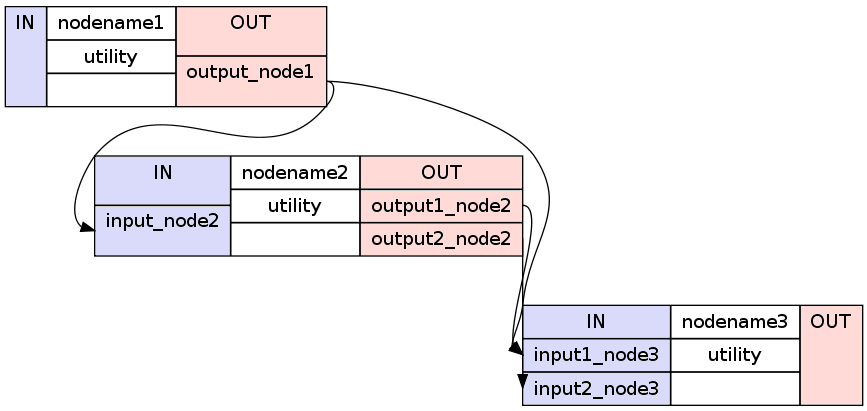
#advanced way to connect multiple nodes
workflowname.connect([(nodename1, nodename2, [('output_node1', 'input_node2')]),
(nodename1, nodename3, [('output_node1', 'input1_node3')]),
(nodename2, nodename3, [('output1_node2', 'input1_node3'),
('output2_node2', 'input2_node3')
])
])
|
It is important to point out that you do not only have to connect the nodes, but rather that you have to connect the output and input fields of each node to the output and input fields of another node.
If you visualize the advanced connection example as a detailed graph, which will be covered in the next section, it would look something as follows:
Sometimes you also want to connect a workflow to another workflow. For example a preprocessing pipeline to a analysis pipeline. This, so that you can execute the whole pipeline as one. To do this, you can’t just connect the nodes to each other. You have to additionally connect the workflows to themselves.
Let’s assume that we have a node realign which is part of a preprocessing pipeline called preprocess and that we have a node called modelspec which is part of an analysis pipeline called modelestimation. To be able to connect those two pipelines at those particular points we need another workflow to serve as a connection scaffold:
1 2 3 4 5 | scaffoldflow = Workflow(name='scaffoldflow')
scaffoldflow.connect([(preprocess, modelestimation,[('realign.out_files',
'modelspec.in_files')
])
])
|
As you see, the main difference to the connections between nodes is that you connect the pipelines first. Nonetheless, you still have to specify which nodes with which output or input fields have to be connected to each other.
There is also the option to add nodes to a workflow without really connecting them to any other nodes or workflow. This can be done with the add_nodes function.
For example
1 2 | #Add smooth and realign to the workflow
workflow.add_nodes([smooth, realign])
|
Sometimes you want to modify the output of one node before sending it on to the next node. This can be done in two ways. Either use an individual node as described above, or plant a function directly between the output and input of two nodes. To do the second approach, do as follows:
First, define your function that modifies the data as you want and returns the new output:
1 2 3 4 | # Define your function that does something special
def myfunction(output_from_node1):
input_for_node2 = output_from_node1 * 2
return input_for_node2
|
Second, insert this function between the connection of the two nodes of interest:
1 2 3 4 | # Insert function between the connection of the two nodes
workflow.connect([(nodename1, nodename2,[(('output_from_node1', myfunction),
'input_for_node2')]),
])
|
This will take the output of output_from_node1 and give it as an argument to the function myfunction. The return value that will be returned by myfunction then will be forwarded as input to input_from_node2.
If you want to insert more than one parameter into the function do as follows:
1 2 3 4 5 6 7 8 9 10 | # Define your function that does something special
def myfunction(output_from_node1, additional_input):
input_for_node2 = output_from_node1 + additional_input
return input_for_node2
# Insert function with additional input between the connection of the two nodes
workflowname.connect([(nodename1,nodename2,[(('out_file_node1', myfunction,
additional_input),
'input_for_node2')]),
])
|
Sometimes you want to reuse a pipeline you’ve already created with some different parameters and node connections. Instead of just copying and changing the whole script, just use the clone command.
For example, if you’ve already created an analysis pipeline that analysis the data on the volume and now would love to reuse this pipeline to do the analysis of the surface, just do as follows:
surfanalysis = volanalysis.clone(name='surfanalysis')
This is all you have to do to have the same connections and parameters in surfanalysis as you have in volanalysis. If you wouldn’t clone the pipeline and keep continuing the same pipeline, Nipype would assume that it still is the same execution flow and just rewrite all the output from the volanalysis pipeline.
If you want to change some parameters of the pipeline after cloning, just specify the name of the pipeline, node and parameter you want to change:
surfanalysis.inputs.level1design.timing_units = 'secs'
This is probably one of the more important and difficult sections of a workflow script, as most of the errors and issues you can encounter with your pipeline are mostly based on some kind of error in the specification of the workflow input or output stream. So make sure that this section is correct.
Before you can tell your computer where it can find your data, you yourself have to understand where and in which format your data is stored at. If you use the tutorial dataset, then your folder structure look as follows:
nipype_tutorial
|-- data
|   |-- sub001
|   |   |-- ...
|   |   |-- run001.nii.gz
|   |   |-- run002.nii.gz
|   |   |-- struct.nii.gz
|   |-- sub002
|   |-- sub003
|-- freesurfer
    |-- sub001
    |-- sub002
    |-- sub003
So this means that your scans are stored in a zipped NIfTI format (i.e. nii.gz) and that you can find them as follows: ~/nipype_tutorial/data/subjectname/scanimage.nii.gz
Now there are two different functions that you can use to specify the folder structure of the input stream. One of them is called SelectFiles and the other one is called DataGrabber. Both are string based and easy to use once understood. Nonetheless, I would recommend to use SelectFiles, as it is much more straight forward to use:
1 2 3 4 5 6 7 8 9 10 11 12 13 14 15 16 17 18 | import nipype.interfaces.io as nio
# SelectFiles
templates = {'anat': 'data/{subject_id}/struct.nii.gz',
'func': 'data/{subject_id}/run*.nii.gz'}
selectfiles = Node(nio.SelectFiles(templates), name="selectfiles")
# DataGrabber
datasource = Node(nio.DataGrabber(infields=['subject_id'],
outfields=['anat', 'func'],
template = 'data/%s/%s.nii'),
name = 'datasource')
info = dict(anat=[['subject_id', 'struct']],
func=[['subject_id', ['run001','run002']]])
datasource.inputs.template_args = info
datasource.inputs.sort_filelist = True
|
Note
Go to the official homepage to read more about DataGrabber and SelectFiles.
In contrast to this, the definition of the output stream is rather simple. You only have to create a DataSink. A DataSink is a node that specifies in which output folder all the relevant results should be stored at.
1 2 3 4 | # Datasink
datasink = Node(nio.DataSink(), name="datasink")
datasink.inputs.base_directory = '~/nipype_tutorial'
datasink.inputs.container = 'datasink_folder'
|
To store an output of a certain node in this DataSink just connect the node to the DataSink. The output data will be saved in the just specified container datasink_folder. Nipype will then save this output in a folder under this container, depending on the name of the DataSink input field that you specify during the creation of connections.
As an example, let’s assume that we want to use the output of SPM’s motion correction node, here called realign.
1 2 3 4 5 6 7 8 | # Saves the realigned files into a subfolder called 'motion'
workflow.connect(realign, datasink, [('realigned_files', 'motion')])
# Saves the realignment_parameters also into the subfolder called 'motion'
workflow.connect(realign, datasink, [('realignment_parameters', 'motion.@par')])
# Saves the realignment parameters in a subfolder 'par', under the folder 'motion'
workflow.connect(realign, datasink, [('realignment_parameters', 'motion.par')])
|
The output folder and files of the datasink node often have long and detailed names, such as '_subject_id_sub002/con_0001_warped_out.nii'. This is because many of the nodes used add their own pre- or postfix to a file or folder. You can use datasink’s substitutions function to change or delete unwanted strings:
1 2 3 4 | # Use the following DataSink output substitutions
substitutions = [('_subject_id_', ''),
('warped_out', 'final')]
datasink.inputs.substitutions = substitutions
|
This substition will change '_subject_id_sub002/con_0001_warped_out.nii' into 'sub002/con_0001_final.nii'.
The DataSink is really useful to keep control over your storage capacity. If you store all the important outputs of your workflow in this folder, you can delete the workflow working directory after executing and counteract storage shortage. You can even set up the configuration of the pipeline so that it will not create a working directory at all. For more information go to Configuration File.
Note
Go to the official homepage to read more about DataSink.
Important
After you’ve created the input and output node it is very important to connect them to the rest of your workflow. Otherwise your pipeline would have no real input or output stream. You can see how to do this in the example below.
After all modules are imported, important variables are specified, nodes are created and connected to workflows, you are able to run your pipeline. This can be done by calling the run() method of the workflow.
As already described in the introduction section, workflows can be run with many different plugins. Those plugins allow you to run your workflow in either normal linear (i.e. sequential) or in parallel ways. Depending on your system, parallel execution is either done on your local machine or on some computation cluster.
Here are just a few example how you can run your workflow:
1 2 3 4 5 6 7 8 9 | # Execute your workflow in sequential way
workflow.run()
# Execute your workflow in parallel.
# Use 4 cores on your local machine
workflow.run('MultiProc', plugin_args={'n_procs': 4})
# Use a cluster environment to run your workflow
workflow.run('SGE', plugin_args={'qsub_args': '-q many'})
|
The computation time of your workflow depends on many different factors, such as which nodes you use, with which parameters, on how many subjects, if you use parallel execution and the power of your system. Therefore, no real prediction about the execution time can be made.
But the nice thing about Nipype is that it will always check if a node has already been run and if the input parameters have changed or not. Only nodes that have different input parameters will be rerun. Nipype’s hashing mechanism ensures that none of the nodes are executed during a new run if the inputs remain the same. This keeps the computation time to its minimum.
Note
More about Plugins and how you can run your pipeline in a distributed system can be found on the official homepage under Using Nipype Plugins.
Let’s try to summarize what we’ve learned by building a short preprocessing pipeline. The following script assumes that you’re using the tutorial dataset with the three subjects sub001, sub002 and sub003, each having two functional scans run001.nii.gz and run002.nii.gz.
First, import all necessary modules. Which modules you have to import becomes clear while you’re adding specific nodes.
1 2 3 4 5 6 7 | from os.path import join as opj
from nipype.interfaces.spm import SliceTiming, Realign, Smooth
from nipype.interfaces.utility import IdentityInterface
from nipype.interfaces.io import SelectFiles, DataSink
from nipype.algorithms.rapidart import ArtifactDetect
from nipype.algorithms.misc import Gunzip
from nipype.pipeline.engine import Workflow, Node
|
Specify all variables that you want to use later in the script. This makes the modification between experiments easy.
1 2 3 4 5 6 7 8 9 10 11 12 13 | experiment_dir = '~/nipype_tutorial' # location of experiment folder
data_dir = opj(experiment_dir, 'data') # location of data folder
fs_folder = opj(experiment_dir, 'freesurfer') # location of freesurfer folder
subject_list = ['sub001', 'sub002', 'sub003'] # list of subject identifiers
session_list = ['run001', 'run002'] # list of session identifiers
output_dir = 'output_firstSteps' # name of output folder
working_dir = 'workingdir_firstSteps' # name of working directory
number_of_slices = 40 # number of slices in volume
TR = 2.0 # time repetition of volume
smoothing_size = 8 # size of FWHM in mm
|
Let’s now create all the nodes we need for this preprocessing workflow:
Gunzip: This node is needed to convert the NIfTI files from the zipped version .nii.gz to the unzipped version .nii. This step has to be done because SPM’s SliceTiming can not handle zipped files.
SliceTiming: This node executes SPM’s SliceTiming on each functional scan.
Realign: This node executes SPM’s Realign on each slice time corrected functional scan.
ArtifactDetect: This node executes ART’s artifact detection on the functional scans.
Smooth: This node executes SPM’s Smooth on each realigned functional scan.
1 2 3 4 5 6 7 8 9 10 11 12 13 14 15 16 17 18 19 20 21 22 23 24 25 26 27 | # Gunzip - unzip functional
gunzip = Node(Gunzip(), name="gunzip")
# Slicetiming - correct for slice wise acquisition
interleaved_order = range(1,number_of_slices+1,2) + range(2,number_of_slices+1,2)
sliceTiming = Node(SliceTiming(num_slices=number_of_slices,
time_repetition=TR,
time_acquisition=TR-TR/number_of_slices,
slice_order=interleaved_order,
ref_slice=2),
name="sliceTiming")
# Realign - correct for motion
realign = Node(Realign(register_to_mean=True),
name="realign")
# Artifact Detection - determine which of the images in the functional series
# are outliers. This is based on deviation in intensity or movement.
art = Node(ArtifactDetect(norm_threshold=1,
zintensity_threshold=3,
mask_type='spm_global',
parameter_source='SPM'),
name="art")
# Smooth - to smooth the images with a given kernel
smooth = Node(Smooth(fwhm=smoothing_size),
name="smooth")
|
Note
Line 5 specifies the slice wise scan acquisition. In our case this was interleaved ascending. Use the following code if you just have ascending (range(1,number_of_slices+1)) or descending (range(number_of_slices,0,-1)).
After we’ve created all the nodes we can create our preprocessing workflow and connect the nodes to this workflow.
1 2 3 4 5 6 7 8 9 10 11 12 13 | # Create a preprocessing workflow
preproc = Workflow(name='preproc')
preproc.base_dir = opj(experiment_dir, working_dir)
# Connect all components of the preprocessing workflow
preproc.connect([(gunzip, sliceTiming, [('out_file', 'in_files')]),
(sliceTiming, realign, [('timecorrected_files', 'in_files')]),
(realign, art, [('realigned_files', 'realigned_files'),
('mean_image', 'mask_file'),
('realignment_parameters',
'realignment_parameters')]),
(realign, smooth, [('realigned_files', 'in_files')]),
])
|
Note
Line 3 is needed to tell the workflow in which folder it should be run. You don’t have to do this for any subworkflows that you’re using. But the “main” workflow, the one which we execute with the .run() command, should always have a base_dir specified.
Before we can run our preprocessing workflow, we first have to specify the input and output stream. To do this, we first have to create the distributor node Infosource, the input node SelectFiles and the output node DataSink. The purpose of Infosource is to tell SelectFiles over which elements of its input stream it should iterate over.
To finish it all up, those three nodes now have to be connected to the rest of the pipeline.
1 2 3 4 5 6 7 8 9 10 11 12 13 14 15 16 17 18 19 20 21 22 23 24 25 26 27 28 29 30 31 32 33 34 35 36 | # Infosource - a function free node to iterate over the list of subject names
infosource = Node(IdentityInterface(fields=['subject_id',
'session_id']),
name="infosource")
infosource.iterables = [('subject_id', subject_list),
('session_id', session_list)]
# SelectFiles
templates = {'func': 'data/{subject_id}/{session_id}.nii.gz'}
selectfiles = Node(SelectFiles(templates,
base_directory=experiment_dir),
name="selectfiles")
# Datasink
datasink = Node(DataSink(base_directory=experiment_dir,
container=output_dir),
name="datasink")
# Use the following DataSink output substitutions
substitutions = [('_subject_id', ''),
('_session_id_', '')]
datasink.inputs.substitutions = substitutions
# Connect SelectFiles and DataSink to the workflow
preproc.connect([(infosource, selectfiles, [('subject_id', 'subject_id'),
('session_id', 'session_id')]),
(selectfiles, gunzip, [('func', 'in_file')]),
(realign, datasink, [('mean_image', 'realign.@mean'),
('realignment_parameters',
'realign.@parameters'),
]),
(smooth, datasink, [('smoothed_files', 'smooth')]),
(art, datasink, [('outlier_files', 'art.@outliers'),
('plot_files', 'art.@plot'),
]),
])
|
Running the pipeline is a rather simple thing. Just use the .run() command with the plugin you want. In our case we want to preprocess the 6 functional scans on 6 cores at once.
1 2 | preproc.write_graph(graph2use='flat')
preproc.run('MultiProc', plugin_args={'n_procs': 6})
|
As you see, we’ve executed the function write_graph() before we’ve run the pipeline. write_graph() is not needed to run the pipeline, but allows you to visualize the execution flow of your pipeline, before you actually execute the pipeline. More about the visualization of workflows can be found in the next chapter, How To Visualize A Pipeline.
Hint
You can download the code for this preprocessing pipeline as a script here: tutorial_3_first_steps.py
After we’ve executed the preprocessing pipeline we have two new folders under ~/nipype_tutorial. The working directory workingdir_firstSteps which contains all files created during the execution of the workflow, and the output folder output_firstSteps which contains all the files that we sent to the DataSink. Let’s take a closer look at those two folders.
The working directory contains many temporary files that might be not so important for your further analysis. That’s why I highly recommend to save all the important outputs of your workflow in a DataSink folder. So that everything important is at one place.
The following folder structure represents the working directory of the above preprocessing workflow:
workingdir_firstSteps
|-- preproc
    |-- _session_id_run001_subject_id_sub001
    |   |-- art
    |   |-- datasink
    |   |-- gunzip
    |   |-- realign
    |   |-- selectfiles
    |   |-- sliceTiming
    |   |-- smooth
    |-- _session_id_run001_subject_id_sub002
    |-- _session_id_run001_subject_id_sub003
    |-- _session_id_run002_subject_id_sub001
    |-- _session_id_run002_subject_id_sub002
    |-- _session_id_run002_subject_id_sub003
Even though the working directory is most often only temporary, it contains many relevant files to be found and explore. Following are some of the highlights:
Visualization: The main folder of the workflow contains the visualized graph files (if created with write_graph() and an interactive execution fiew (index.html).
Reports: Each node contains a subfolder called _report that contains a file called report.rst. This file contains all relevant node information. E.g. What’s the name of the node and what is its hierarchical place in the pipeline structure? What are the actual input and executed output parameters? How long did it take to execute the node and what were the values of the environment variables during the execution?
The output folder contains exactly the files that we sent to the DataSink. Each node contains its own folder and in each of those folder a subfolder for each subject is created.
output_firstSteps
|-- art
|   |-- run001_sub001
|   |   |-- art.rarun001_outliers.txt
|   |   |-- plot.rarun001.png
|   |-- run001_sub002
|   |-- run001_sub003
|   |-- run002_sub001
|   |-- run002_sub002
|   |-- run002_sub003
|-- realign
|   |-- run001_sub001
|   |   |-- meanarun001.nii
|   |   |-- rp_arun001.txt
|   |-- run001_sub002
|   |-- run001_sub003
|   |-- run002_sub001
|   |-- run002_sub002
|   |-- run002_sub003
|-- smooth
    |-- run001_sub001
    |   |-- srarun001.nii
    |-- run001_sub002
    |-- run001_sub003
    |-- run002_sub001
    |-- run002_sub002
    |-- run002_sub003
The goal of this output folder is to store all important outputs in this folder. This allows you to delete the working directory and get rid of its many unnecessary temporary files.
As so often in life, there is always something that doesn’t go as planed. And this is the same for Nipype. There are many reasons why a pipeline can cause problems or even crash. But there’s always a way to figure out what went wrong and what needs to be fixed.
Before we take a look at how to find errors, let’s take a look at a correct working pipeline. The following is the abbreviated terminal output of the preprocessing workflow from above. For readability reasons, lines containing the execution timestamps are not shown:
1 2 3 4 5 6 7 8 9 10 11 12 13 14 15 16 17 18 19 20 21 22 23 24 25 26 27 28 29 30 31 | ['check', 'execution', 'logging']
Running in parallel.
Submitting 3 jobs
Executing: selectfiles.a2 ID: 0
Executing: selectfiles.a1 ID: 1
Executing: selectfiles.a0 ID: 14
Executing node selectfiles.a2 in dir: ~/nipype_tutorial/workingdir_firstSteps/
preproc/_subject_id_sub003/selectfiles
Executing node selectfiles.a1 in dir: ~/nipype_tutorial/workingdir_firstSteps/
preproc/_subject_id_sub002/selectfiles
Executing node selectfiles.a0 in dir: ~/nipype_tutorial/workingdir_firstSteps/
preproc/_subject_id_sub001/selectfiles
[Job finished] jobname: selectfiles.a2 jobid: 0
[Job finished] jobname: selectfiles.a1 jobid: 1
[Job finished] jobname: selectfiles.a0 jobid: 14
[...]
Submitting 3 jobs
Executing: datasink.a1 ID: 7
Executing: datasink.a2 ID: 13
Executing: datasink.a0 ID: 20
Executing node datasink.a0 in dir: ~/nipype_tutorial/workingdir_firstSteps/
preproc/_subject_id_sub001/datasink
Executing node datasink.a1 in dir: ~/nipype_tutorial/workingdir_firstSteps/
preproc/_subject_id_sub002/datasink
Executing node datasink.a2 in dir: ~/nipype_tutorial/workingdir_firstSteps/
preproc/_subject_id_sub003/datasink
[Job finished] jobname: datasink.a1 jobid: 7
[Job finished] jobname: datasink.a2 jobid: 13
[Job finished] jobname: datasink.a0 jobid: 20
|
This output shows you the chronological execution of the pipeline, run in parallel mode. Each node first has to be transformed into a job and submitted to the execution cluster. The start of a node’s execution is accompanied by the working directory of this node. The output [Job finished] then tells you when the execution of the node is done.
In the beginning when you’re not used to reading Nipype’s terminal output it can be tricky to find the actual error. But most of the time, Nipype tells you exactly what’s wrong.
Let’s assume for example, that you want to create a preprocessing pipeline as shown above but forget to provide the mandatory input realigned_files for the artifact detection node art. The running of such a workflow will lead to the following terminal output:
1 2 3 4 5 6 7 8 9 10 11 12 13 14 15 16 17 18 19 20 21 22 23 24 25 26 27 28 29 30 31 32 33 34 35 36 37 38 39 40 41 42 43 44 45 46 47 48 49 50 51 52 53 54 | 141018-14:01:51,671 workflow INFO:
['check', 'execution', 'logging']
141018-14:01:51,688 workflow INFO:
Running serially.
141018-14:01:51,689 workflow INFO:
Executing node selectfiles.b0 in dir: ~/nipype_tutorial/workingdir_firstSteps/
preproc/_subject_id_sub001/selectfiles
141018-14:01:51,697 workflow INFO:
Executing node gunzip.b0 in dir: ~/nipype_tutorial/workingdir_firstSteps/
preproc/_subject_id_sub001/gunzip
141018-14:01:51,699 workflow INFO:
Executing node _gunzip0 in dir: ~/nipype_tutorial/workingdir_firstSteps/
preproc/_subject_id_sub001/gunzip/mapflow/_gunzip0
141018-14:01:52,53 workflow INFO:
Executing node sliceTiming.b0 in dir: ~/nipype_tutorial/workingdir_firstSteps/
preproc/_subject_id_sub001/sliceTiming
141018-14:02:30,30 workflow INFO:
Executing node realign.b0 in dir: ~/nipype_tutorial/workingdir_firstSteps/
preproc/_subject_id_sub001/realign
141018-14:03:29,374 workflow INFO:
Executing node smooth.aI.a1.b0 in dir: ~/nipype_tutorial/workingdir_firstSteps/
preproc/_subject_id_sub001/smooth
141018-14:04:40,927 workflow INFO:
Executing node art.b0 in dir: ~/nipype_tutorial/workingdir_firstSteps/
preproc/_subject_id_sub001/art
141018-14:04:40,929 workflow ERROR:
['Node art.b0 failed to run on host mnotter.']
141018-14:04:40,930 workflow INFO:
Saving crash info to ~/nipype_tutorial/crash-20141018-140440-mnotter-art.b0.pklz
141018-14:04:40,930 workflow INFO:
Traceback (most recent call last):
File "~/anaconda/lib/python2.7/site-packages/nipype/pipeline/plugins/linear.py",
line 38, in run node.run(updatehash=updatehash)
File "~/anaconda/lib/python2.7/site-packages/nipype/pipeline/engine.py",
line 1424, in run self._run_interface()
File "~/anaconda/lib/python2.7/site-packages/nipype/pipeline/engine.py",
line 1534, in _run_interface self._result = self._run_command(execute)
File "~/anaconda/lib/python2.7/site-packages/nipype/pipeline/engine.py",
line 1660, in _run_command result = self._interface.run()
File "~/anaconda/lib/python2.7/site-packages/nipype/interfaces/base.py",
line 965, in run self._check_mandatory_inputs()
File "~/anaconda/lib/python2.7/site-packages/nipype/interfaces/base.py",
line 903, in _check_mandatory_inputs raise ValueError(msg)
ValueError: ArtifactDetect requires a value for input 'realigned_files'.
For a list of required inputs, see ArtifactDetect.help()
141018-14:05:18,144 workflow INFO:
***********************************
141018-14:05:18,144 workflow ERROR:
could not run node: preproc.art.b0
141018-14:05:18,144 workflow INFO:
crashfile: ~/nipype_tutorial/crash-20141018-140440-mnotter-art.b0.pklz
141018-14:05:18,144 workflow INFO:
***********************************
|
Now, what happened? Line 26 indicates you that there is an Error and line 29 tells you where the crash report to this error was saved at. The last part of this crash file (i.e. art.b0.pklz) tells you that the error happened in the art node. Line 31-43 show the exact error stack of the current crash. Those multiple lines starting with File are also always a good indicator to find the error in the terminal output.
Now the important output is shown in line 44. Here it actually tells you what is wrong. ArtifactDetect requires a value for input 'realigned_files'. Correct this issue and the workflow should execute cleanly.
Always at the end of the output is a section that summarizes the whole crash. In this case this is line 48-54. Here you can see again which nodes lead to the crash and where the crash file to the error is stored at.
But sometimes, just knowing where and because of what the crash happened is not enough. You also need to know what the actual values of the crashed nodes were, to see if perhaps some input values were not transmitted correctly.
This can be done with the shell command nipype_display_crash. To read for example the above mentioned art-crash file, we have to open a new terminal and run the following command:
nipype_display_crash ~/nipype_tutorial/crash-20141018-140857-mnotter-art.b0.pklz
This will lead to the following output:
1 2 3 4 5 6 7 8 9 10 11 12 13 14 15 16 17 18 19 20 21 22 23 24 25 26 27 28 29 30 31 32 33 34 35 36 37 38 39 40 41 42 | File: crash-20141018-140857-mnotter-art.b0.pklz
Node: preproc.art.b0
Working directory: ~/nipype_tutorial/workingdir_firstSteps/
preproc/_subject_id_sub001/art
Node inputs:
bound_by_brainmask = False
global_threshold = 8.0
ignore_exception = False
intersect_mask = <undefined>
mask_file = <undefined>
mask_threshold = <undefined>
mask_type = spm_global
norm_threshold = 0.5
parameter_source = SPM
plot_type = png
realigned_files = <undefined>
realignment_parameters = ['~/nipype_tutorial/workingdir_firstSteps/preproc/
_subject_id_sub001/realign/rp_arun001.txt']
rotation_threshold = <undefined>
save_plot = True
translation_threshold = <undefined>
use_differences = [True, False]
use_norm = True
zintensity_threshold = 3.0
Traceback (most recent call last):
File "~/anaconda/lib/python2.7/site-packages/nipype/pipeline/plugins/linear.py",
line 38, in run node.run(updatehash=updatehash)
File "~/anaconda/lib/python2.7/site-packages/nipype/pipeline/engine.py",
line 1424, in run self._run_interface()
File "~/anaconda/lib/python2.7/site-packages/nipype/pipeline/engine.py",
line 1534, in _run_interface self._result = self._run_command(execute)
File "~/anaconda/lib/python2.7/site-packages/nipype/pipeline/engine.py",
line 1660, in _run_command result = self._interface.run()
File "~/anaconda/lib/python2.7/site-packages/nipype/interfaces/base.py",
line 965, in run self._check_mandatory_inputs()
File "~/anaconda/lib/python2.7/site-packages/nipype/interfaces/base.py",
line 903, in _check_mandatory_inputs raise ValueError(msg)
ValueError: ArtifactDetect requires a value for input 'realigned_files'.
For a list of required inputs, see ArtifactDetect.help()
|
From this output you can see in the lower half the same error stack of the crash and the exact description of what is wrong, as we’ve seen in the terminal output. But in the first half you also have additional information of the nodes input, which might help to solve some problems.
Note
Note that the information about the exact input values of a node can also be obtained from the report.rst file, stored in the nodes subfolder under the working directory. More about this later under Working Directory.
Sometimes the most basic errors can occur because Nipype doesn’t know where the correct files are. Two very common issues are for example that FreeSurfer can’t find the subject folder or that MATLAB doesn’t find SPM.
Before you do anything else, please make sure again that you’ve installed FreeSurfer and SPM12 as described in the installation section, How to install FreeSurfer and How to install SPM.
But don’t worry if the problem still exists. There are two nice ways how you can tell Nipype where FreeSurfer subject folders are stored at and where MATLAB can find SPM12. Just add the following code to the beginning of your script:
1 2 3 4 5 6 7 | # Import FreeSurfer and specify the path to the current subject directory
import nipype.interfaces.freesurfer as fs
fs.FSCommand.set_default_subjects_dir('~/nipype_tutorial/freesurfer')
# Import MATLAB command and specify the path to SPM12
from nipype.interfaces.matlab import MatlabCommand
MatlabCommand.set_default_paths('/usr/local/MATLAB/R2014a/toolbox/spm12')
|
Sometimes the biggest issue with your code is that you try to force things that can’t work.
One common example is that you try to feed in two values (e.g. run001 and run002) into an input field that only expects one value. An example output of such an Error would contain something like this:
1 2 3 | TraitError: The 'in_file' trait of a GunzipInputSpec instance must be an existing file
name, but a value of ['~/nipype_tutorial/data/sub002/run001.nii.gz',
'~/nipype_tutorial/data/sub002/run002.nii.gz'] <type 'list'> was specified.
|
This error tells you that it expects an 'in_file' (i.e. singular) and that the file ['run001', 'run002'] doesn’t exist. What makes sense, because a list isn’t a file. Such an error can often times be resolved by using a MapNode. Otherwise, find another way to reduce the number of input values per field.
Another common mistake is the fact that your data is given as input to a node that can’t handle the format of this input. This error is most often encountered when your data type is zipped and the following node can’t unzip the file by itself. We included a Gunzip node exaclty for this reason in the example pipeline above.
So what will the terminal output look like if we try to feed a zipped run001.nii.gz to a node that executes SPM’s SliceTiming?
1 2 3 4 5 6 7 8 9 10 11 12 13 14 15 16 17 18 19 20 21 22 23 24 25 26 27 28 29 30 31 32 33 34 35 36 37 38 39 40 41 42 43 44 45 46 47 48 49 50 51 52 53 54 55 | 141018-13:25:22,227 workflow INFO:
Executing node selectfiles.b0 in dir: ~/nipype_tutorial/workingdir_firstSteps/
preproc/_subject_id_sub001/selectfiles
141018-13:25:22,235 workflow INFO:
Executing node sliceTiming.b0 in dir: ~/nipype_tutorial/workingdir_firstSteps/
preproc/_subject_id_sub001/sliceTiming
141018-13:25:39,673 workflow ERROR:
['Node sliceTiming.b0 failed to run on host mnotter.']
141018-13:25:39,673 workflow INFO:
Saving crash info to ~/nipype_tutorial/
crash-20141018-132539-mnotter-sliceTiming.b0.pklz
[...]
< M A T L A B (R) >
Copyright 1984-2014 The MathWorks, Inc.
R2014a (8.3.0.532) 64-bit (glnxa64)
February 11, 2014
[...]
Warning: Run spm_jobman('initcfg'); beforehand
> In spm_jobman at 106
In pyscript_slicetiming at 362
Item 'Session', field 'val': Number of matching files (0) less than required (2).
Item 'Session', field 'val': Number of matching files (0) less than required (2).
Standard error:
MATLAB code threw an exception:
No executable modules, but still unresolved dependencies or incomplete module inputs.
File:/usr/local/MATLAB/R2014a/toolbox/spm12/spm_jobman.m
Name:/usr/local/MATLAB/R2014a/toolbox/spm12/spm_jobman.m
Line:47
File:~/nipype_tutorial/workingdir_firstSteps/preproc/
_subject_id_sub001/sliceTiming/pyscript_slicetiming.m
Name:fill_run_job
Line:115
File:pm_jobman
Name:pyscript_slicetiming
Line:459
File:ç
Name:U
Line:
Return code: 0
Interface MatlabCommand failed to run.
Interface SliceTiming failed to run.
141018-13:25:39,681 workflow INFO:
***********************************
141018-13:25:39,682 workflow ERROR:
could not run node: preproc.sliceTiming
141018-13:25:39,682 workflow INFO:
crashfile: ~/nipype_tutorial/crash-20141018-132539-mnotter-sliceTiming.pklz
141018-13:25:39,682 workflow INFO:
***********************************
|
This error message doesn’t tell you directly what is wrong. Unfortunately, Nipype can’t go deep enough into SPM’s code and figure out what is wrong, because SPM itself doesn’t tell us what’s wrong. But line 25-26 tells us that SPM has some issues with finding the appropriate files.
Hint
For more information about Errors go to the Support section of this beginner’s guide.