Nipype Quickstart¶

Nipype architecture

Existing documentation
Visualizing the evolution of Nipype
This notebook is taken from reproducible-imaging repository

Import a few things from nipype and external libraries¶

import os
from os.path import abspath

from nipype import Workflow, Node, MapNode, Function
from nipype.interfaces.fsl import BET, IsotropicSmooth, ApplyMask

from nilearn.plotting import plot_anat
%matplotlib inline
import matplotlib.pyplot as plt

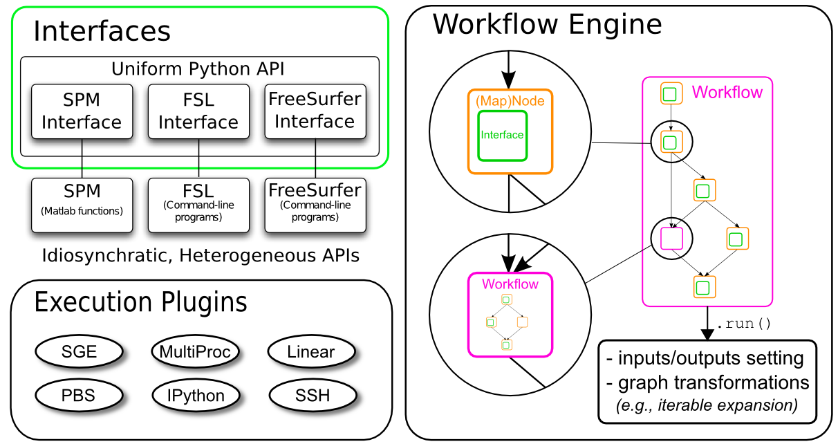
Interfaces¶

Interfaces are the core pieces of Nipype. The interfaces are python modules that allow you to use various external packages (e.g. FSL, SPM or FreeSurfer), even if they themselves are written in another programming language than python.

Let's try to use bet from FSL:

# will use a T1w from ds000114 dataset
input_file =  abspath("/data/ds000114/sub-01/ses-test/anat/sub-01_ses-test_T1w.nii.gz")

# we will be typing here

If you're lost the code is here:

bet = BET()
bet.inputs.in_file = input_file
bet.inputs.out_file = "/output/T1w_nipype_bet.nii.gz"
res = bet.run()

let's check the output:

res.outputs

and we can plot the output file

plot_anat('/output/T1w_nipype_bet.nii.gz', 
          display_mode='ortho', dim=-1, draw_cross=False, annotate=False);

you can always check the list of arguments using help method

BET.help()

Exercise 1a¶

Import IsotropicSmooth from nipype.interfaces.fsl and find out the FSL command that is being run. What are the mandatory inputs for this interface?

# type your code here

from nipype.interfaces.fsl import IsotropicSmooth
# all this information can be found when we run `help` method. 
# note that you can either provide `in_file` and `fwhm` or `in_file` and `sigma`
IsotropicSmooth.help()

Exercise 1b¶

Run the IsotropicSmooth for /data/ds000114/sub-01/ses-test/anat/sub-01_ses-test_T1w.nii.gz file with a smoothing kernel 4mm:

# type your solution here

smoothing = IsotropicSmooth()
smoothing.inputs.in_file = "/data/ds000114/sub-01/ses-test/anat/sub-01_ses-test_T1w.nii.gz"
smoothing.inputs.fwhm = 4
smoothing.inputs.out_file = "/output/T1w_nipype_smooth.nii.gz"
smoothing.run()

# plotting the output
plot_anat('/output/T1w_nipype_smooth.nii.gz', 
          display_mode='ortho', dim=-1, draw_cross=False, annotate=False);

Nodes and Workflows¶

Interfaces are the core pieces of Nipype that run the code of your desire. But to streamline your analysis and to execute multiple interfaces in a sensible order, you have to put them in something that we call a Node and create a Workflow.

In Nipype, a node is an object that executes a certain function. This function can be anything from a Nipype interface to a user-specified function or an external script. Each node consists of a name, an interface, and at least one input field and at least one output field.

Once you have multiple nodes you can use Workflow to connect with each other and create a directed graph. Nipype workflow will take care of input and output of each interface and arrange the execution of each interface in the most efficient way.

Let's create the first node using BET interface:

# we will be typing here

If you're lost the code is here:

# Create Node
bet_node = Node(BET(), name='bet')
# Specify node inputs
bet_node.inputs.in_file = input_file
bet_node.inputs.mask = True

# bet node can be also defined this way:
#bet_node = Node(BET(in_file=input_file, mask=True), name='bet_node')

Exercise 2¶

Create a Node for IsotropicSmooth interface.

# Type your solution here:

# smooth_node =

smooth_node = Node(IsotropicSmooth(in_file=input_file, fwhm=4), name="smooth")

We will now create one more Node for our workflow

mask_node = Node(ApplyMask(), name="mask")

Let's check the interface:

ApplyMask.help()

As you can see the interface takes two mandatory inputs: in_file and mask_file. We want to use the output of smooth_node as in_file and one of the output of bet_file (the mask_file) as mask_file input.

Let's initialize a Workflow:

# will be writing the code here:

if you're lost, the full code is here:

# Initiation of a workflow
wf = Workflow(name="smoothflow", base_dir="/output/working_dir")

It's very important to specify base_dir (as absolute path), because otherwise all the outputs would be saved somewhere in the temporary files.

let's connect the bet_node output to mask_node input`

# we will be typing here:

if you're lost, the code is here:

wf.connect(bet_node, "mask_file", mask_node, "mask_file")

Exercise 3¶

Connect out_file of smooth_node to in_file of mask_node.

# type your code here

wf.connect(smooth_node, "out_file", mask_node, "in_file")

Let's see a graph describing our workflow:

wf.write_graph("workflow_graph.dot")
from IPython.display import Image
Image(filename="/output/working_dir/smoothflow/workflow_graph.png")

you can also plot a more detailed graph:

wf.write_graph(graph2use='flat')
from IPython.display import Image
Image(filename="/output/working_dir/smoothflow/graph_detailed.png")

and now let's run the workflow

# we will type our code here:

if you're lost, the full code is here:

# Execute the workflow
res = wf.run()

and let's look at the results

# we can check the output of specific nodes from workflow
list(res.nodes)[0].result.outputs

we can see the fie structure that has been created:

! tree -L 3 /output/working_dir/smoothflow/

and we can plot the results:

import numpy as np
import nibabel as nb
#import matplotlib.pyplot as plt

# Let's create a short helper function to plot 3D NIfTI images
def plot_slice(fname):

    # Load the image
    img = nb.load(fname)
    data = img.get_data()

    # Cut in the middle of the brain
    cut = int(data.shape[-1]/2) + 10

    # Plot the data
    plt.imshow(np.rot90(data[..., cut]), cmap="gray")
    plt.gca().set_axis_off()

f = plt.figure(figsize=(12, 4))
for i, img in enumerate(["/data/ds000114/sub-01/ses-test/anat/sub-01_ses-test_T1w.nii.gz",
                         "/output/working_dir/smoothflow/smooth/sub-01_ses-test_T1w_smooth.nii.gz",
                         "/output/working_dir/smoothflow/bet/sub-01_ses-test_T1w_brain_mask.nii.gz",
                         "/output/working_dir/smoothflow/mask/sub-01_ses-test_T1w_smooth_masked.nii.gz"]):
    f.add_subplot(1, 4, i + 1)
    plot_slice(img)

Iterables¶

Some steps in a neuroimaging analysis are repetitive. Running the same preprocessing on multiple subjects or doing statistical inference on multiple files. To prevent the creation of multiple individual scripts, Nipype has as execution plugin for Workflow, called iterables.

Let's assume we have a workflow with two nodes, node (A) does simple skull stripping, and is followed by a node (B) that does isometric smoothing. Now, let's say, that we are curious about the effect of different smoothing kernels. Therefore, we want to run the smoothing node with FWHM set to 2mm, 8mm, and 16mm.

let's just modify smooth_node:

# we will type the code here

if you're lost the code is here:

smooth_node_it = Node(IsotropicSmooth(in_file=input_file), name="smooth")
smooth_node_it.iterables = ("fwhm", [4, 8, 16])

we will define again bet and smooth nodes:

bet_node_it = Node(BET(in_file=input_file, mask=True), name='bet_node')
mask_node_it = Node(ApplyMask(), name="mask")

will create a new workflow with a new base_dir:

# Initiation of a workflow
wf_it = Workflow(name="smoothflow_it", base_dir="/output/working_dir")
wf_it.connect(bet_node_it, "mask_file", mask_node_it, "mask_file")
wf_it.connect(smooth_node_it, "out_file", mask_node_it, "in_file")

let's run the workflow and check the output

res_it = wf_it.run()

let's see the graph

list(res_it.nodes)

We can see the file structure that was created:

! tree -L 3 /output/working_dir/smoothflow_it/

you have now 7 nodes instead of 3!

MapNode¶

If you want to iterate over a list of inputs, but need to feed all iterated outputs afterward as one input (an array) to the next node, you need to use a MapNode. A MapNode is quite similar to a normal Node, but it can take a list of inputs and operate over each input separately, ultimately returning a list of outputs.

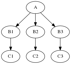
Imagine that you have a list of items (let's say files) and you want to execute the same node on them (for example some smoothing or masking). Some nodes accept multiple files and do exactly the same thing on them, but some don't (they expect only one file). MapNode can solve this problem. Imagine you have the following workflow:

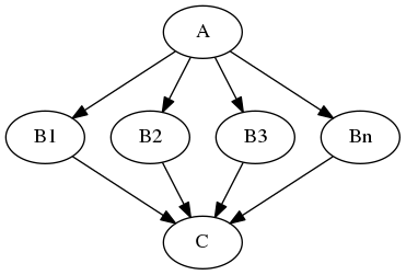
Node A outputs a list of files, but node B accepts only one file. Additionally, C expects a list of files. What you would like is to run B for every file in the output of A and collect the results as a list and feed it to C.

Let's run a simple numerical example using nipype Function interface

def square_func(x):
    return x ** 2

square = Function(input_names=["x"], output_names=["f_x"], function=square_func)

If I want to know the results only for one x we can use Node:

square_node = Node(square, name="square")
square_node.inputs.x = 2
res = square_node.run()
res.outputs

let's try to ask for more values of x

# NBVAL_SKIP
square_node = Node(square, name="square")
square_node.inputs.x = [2, 4]
res = square_node.run()
res.outputs

It will give an error since square_func do not accept list. But we can try MapNode:

square_mapnode = MapNode(square, name="square", iterfield=["x"])
square_mapnode.inputs.x = [2, 4]
res = square_mapnode.run()
res.outputs

Notice that f_x is a list again!