Important
This guide hasn’t been updated since January 2017 and is based on an older version of Nipype. The code in this guide is not tested against newer Nipype versions and might not work anymore. For a newer, more up to date and better introduction to Nipype, please check out the the Nipype Tutorial.
In this section, I will introduce you to the basics of analyzing neuroimaging data. I will give a brief explanation of how the neuroimaging data is acquired, how the data is prepared for analysis (also called preprocessing). Finally, I’ll show how you can analyze your data using a model based on your hypothesis.
Note
This part is only a brief introduction to neuroimaging. Further information on this topic can be found under the Glossary and FAQ pages of this beginner’s guide.
The technology and physics behind an MRI scanner is quite astonishing. But I won’t go into the details of how it all works. You do need to know some terms, concepts, and parameters that are used to acquire MRI data in a scanning session and use that to construct useable images.
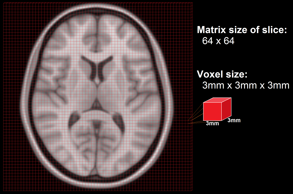
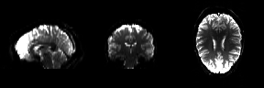
The brain occupies space, so when we collect data on how it fills space, we call that volume data, and all the volume data needed to create the complete, 3D image of the brain, recorded at one single timepoint and as pictured on the left, is called a volume. The data is measured in voxels, which are like the pixels used to display images on your screen, only in 3D. Each voxel has a specific dimension, in this case it is 1mm x 1mm x 1mm: a cube, so it is the same dimension from all sides (isotropic). Each voxel contains one value which stands for the average signal measured at the given location.
A standard anatomical volume, with an isotropic voxel resolution of 1mm contains almost 17 million voxels, which are arranged in a 3D matrix of 256 x 256 x 256 voxels. The following picture shows a slice – one layer of the big, 3D matrix – through a brain volume, and the superimposed grid shows the remaining two dimensions of the voxels.
As the scanner can’t measure the whole volume at once it has to measure portions of the brain sequentially in time. This is done by measuring one plane of the brain (generally the horizontal one) after the other. Such a plane is also called a slice. The resolution of the measured volume data, therefore, depends on the in-plane resolution (the size of the squares in the above image), the number of slices and their thickness (how many layers), and any possible gaps between the layers.
The quality of the measured data depends on the resolution and the following parameters:
repetition time (TR): time required to scan one volume
acquisition time (TA): time required to scan one slice. TA = TR - (TR/number of slices)
field of view (FOV): defines the extent of a slice, e.g. 256mm x 256mm
MRI scanners output their neuroimaging data in a raw data format with which most analysis packages cannot work. DICOM is a common, standardized, raw medical image format, but the format of your raw data may be something else; e.g., PAR/REC format from Philips scanners. Raw data is saved in k-space format, and it needs to be converted into a format that the analysis packages can use. The most frequent format for newly generated data is called NIfTI. If you are working with older datasets, you may encounter data in Analyze format. MRI data formats will have an image and a header part. For NifTI format, they are in the same file (.nii-file), whereas in the older Analyze format, they are in separate files (.img and .hdr-file).
The image is the actual data and is represented by a 3D matrix that contains a value (e.g. gray value) for each voxel.
The header contains information about the data like voxel dimension, voxel extend in each dimension, number of measured time points, a transformation matrix that places the 3D matrix from the image part in a 3D coordinate system, etc.
There are many different kinds of acquisition techniques. But the most common ones are structural magnetic resonance imaging (sMRI), functional magnetic resonance imaging (fMRI) and diffusion tensor imaging (DTI).
Structural magnetic resonance imaging (sMRI) is a technique for measuring the anatomy of the brain. By measuring the amount of water at a given location, sMRI is capable of acquiring a detailed anatomical picture of our brain. This allows us to accurately distinguish between different types of tissue, such as gray and white matter. Structural images are high-resolution images of the brain that are used as reference images for multiple purposes, such as corregistration, normalization, segmentation, and surface reconstruction.
As there is no time pressure during acquisition of anatomical images (the anatomy is not supposed to change while the person is in the scanner), a higher resolution can be used for recording anatomical images, with a voxel extent of 0.2 to 1.5mm, depending on the strength of the magnetic field in the scanner, e.g. 1.5T, 3T or 7T. Grey matter structures are seen in dark, and the white matter structures in bright colors.
Functional magnetic resonance imaging (fMRI) is a technique for measuring brain activity. It works by detecting the changes in blood oxygenation and blood flow that occur in response to neural activity. Our brain is capable of so many astonishing things. But as nothing comes from nothing, it needs a lot of energy to sustain its functionality, and increased activity at a location increases the local energy consumption in the form of oxygen (O2) which is carried by the blood. Therefore, increased function results in increased blood flow towards the energy consuming location.
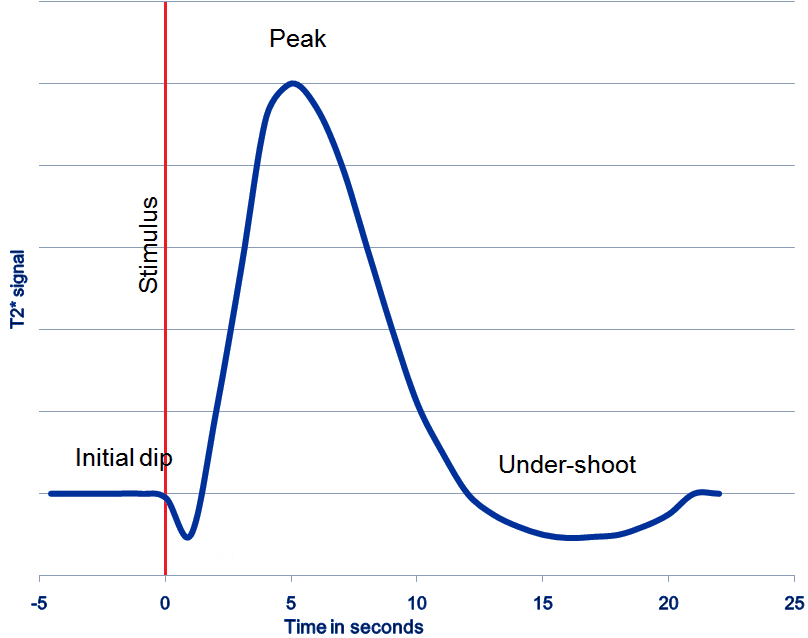
Immediately after neural activity the blood oxygen level decreases, known as the initial dip, because of the local energy consumption. This is followed by increased flow of new and oxygen-rich blood towards the energy consuming region. After 4-6 seconds a peak of blood oxygen level is reached. After no further neuronal activation takes place the signal decreases again and typically undershoots, before rising again to the baseline level.
The blood oxygen level is exactly what we measure with fMRI. The MRI Scanner is able to measure the changes in the magnetic field caused by the difference in the magnetic susceptibility of oxygenated (diamagnetic) and deoxygenated (paramagnetic) blood. The signal is therefore called the Blood Oxygen Level Dependent (BOLD) response.
Because the BOLD signal has to be measured quickly, the resolution of functional images is normally lower (2-4mm) than the resolution of structural images (0.5-1.5mm). But this depends strongly on the strength of the magnetic field in the scanner, e.g. 1.5T, 3T or 7T. In a functional image, the gray matter is seen as bright and the white matter as dark colors, which is the exact opposite to structural images.
Depending on the paradigm, we talk about event-related, block or resting-state designs.
event-related design: Event-related means that stimuli are administered to the subjects in the scanner for a short period. The stimuli are only administered briefly and generally in random order. Stimuli are typically visual, but audible or or other sensible stimuli could also be used. This means that the BOLD response consists of short bursts of activity, which should manifest as peaks, and should look more or less like the line shown in the graph above.
block design: If multiple stimuli of a similar nature are shown in a block, or phase, of 10-30 seconds, that is a block design. Such a design has the advantages that the peak in the BOLD signal is not just attained for a short period but elevated for a longer time, creating a plateau in the graph. This makes it easier to detect an underlying activation increase.
resting-state design: Resting-state designs acquire data in the absence of stimulation. Subjects are asked to lay still and rest in the scanner without falling asleep. The goal of such a scan is to record brain activation in the absence of an external task. This is sometimes done to analyze the functional connectivity of the brain.
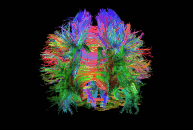
Diffusion imaging is done to obtain information about the brain’s white matter connections. There are multiple modalities to record diffusion images, such as diffusion tensor imaging (DTI), diffusion spectrum imaging (DSI), diffusion weighted imaging (DWI) and diffusion functional MRI (DfMRI). By recording the diffusion trajectory of the molecules (usually water) in a given voxel, one can make inferences about the underlying structure in the voxel. For example, if one voxel contains mostly horizontal fiber tracts, the water molecules in this region will mostly diffuse (move) in a horizontal manner, as they can’t move vertically because of this neural barrier. The diffusion itself is mostly a Brownian motion.
There are many different diffusion measurements, such as mean diffusivity (MD), fractional anisotropy (FA) and Tractography. Each measurement gives different insights into the brain’s neural fiber tracts. An example of a reconstructed tractography can be seen in the image to the left.
Diffusion MRI is a rather new field in MRI and still has some problems with its sensitivity to correctly detect fiber tracts and their underlying orientation. For example, the standard DTI method has almost no chance of reliably detecting kissing (touching) or crossing fiber tracts. To account for this disadvantage, newer methods such as High-angular-resolution diffusion imaging (HARDI) and Q-ball vector analysis were developed. For more about diffusion MRI see the Diffusion MRI Wikipedia page.
There are many different steps involved in a neuroimaging analysis and there is not just one order in which to perform them. Depending on the researcher, the paradigm at hand, or the modality analyzed (sMRI, fMRI, dMRI), the order can differ. Some steps may occur earlier or later or may be left out entirely. Nonetheless, the general procedure for fMRI analysis can be divided into the following three steps:
Preprocessing: Spatial and temporal preprocessing of the data to prepare it for the 1st and 2nd level inferential analysis
Model Specification and Estimation: Specifying and estimating parameters of the statistical model
Statistical Inference: Making inferences about the estimated parameters using appropriate statistical methods
Preprocessing is the term used to for all the steps taken to improve our data and prepare it for statistical analysis. We may correct or adjust our data for a number of things inherent in the experimental situation: to take account of time differences between acquiring each image slice, to correct for head movement during scanning, to detect ‘artifacts’ – anomalous measurements – that should be excluded from subsequent analysis; to align the functional images with the reference structural image, and to normalize the data into a standard space so that data can be compared among several subjects; to apply filtering to the image to increase the signal-to-noise ratio; finally, if sMRI is intended, a segmentation step may be performed. We will now look at each of those steps in more detail.

Because functional MRI measurement sequences don’t acquire every slice in a volume at the same time we have to account for the time differences among the slices. For example, if you acquire a volume with 37 slices in ascending order, and each slice is acquired every 50ms, there is a difference of 1.8s between the first and the last slice acquired. You must know the order in which the slices were acquired to be able to apply the proper correction. Slices are typically acquired in one of three methods: descending order (top-down); ascending order (bottom-up); or interleaved (acquire every other slice in each direction), where the interleaving may start at the top or the bottom. (Left: ascending, Right: interleaved)
Slice Timing Correction is used to compensate for the time differences between the slice acquisitions by temporally interpolating the slices so that the resulting volume is close to equivalent to acquiring the whole brain image at a single time point. This temporal factor of acquisition especially has to be accounted for in fMRI models where timing is an important factor (e.g. for event related designs, where the type of stimulus changes from volume to volume).
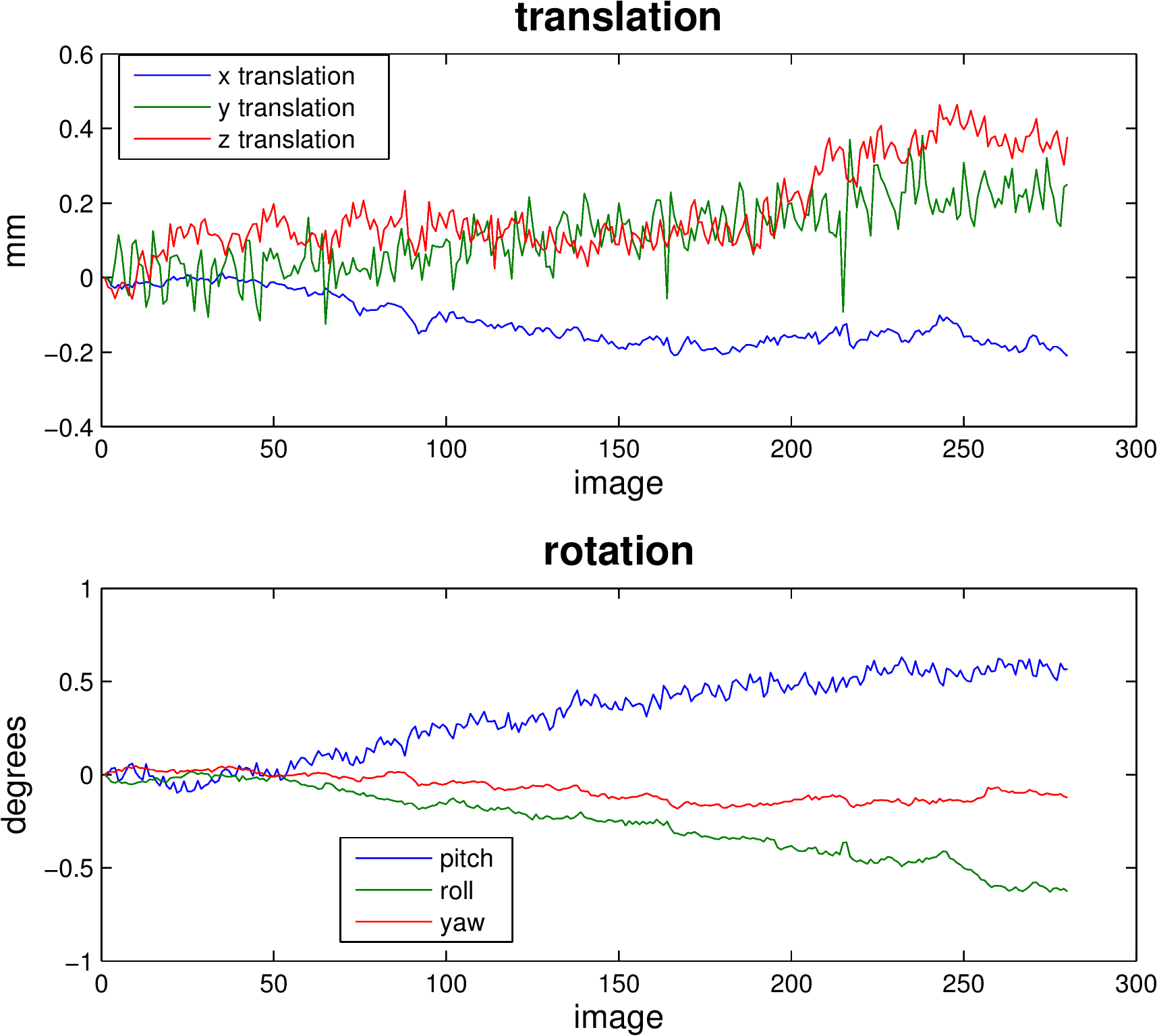
Motion correction, also known as Realignment, is used to correct for head movement during the acquisition of functional data. Even small head movements lead to unwanted variation in voxels and reduce the quality of your data. Motion correction tries to minimize the influence of movement on your data by aligning your data to a reference time volume. This reference time volume is usually the mean image of all timepoints, but it could also be the first, or some other, time point.
Head movement can be characterized by six parameters: Three translation parameters which code movement in the directions of the three dimensional axes, movement along the X, Y, or Z axes; and three rotation parameters which code rotation about those axes, rotation centered on each of the X, Y, and Z axes).
Realignment usually uses an affine rigid body transformation to manipulate the data in those six parameters. That is, each image can be moved but not distorted to best align with all the other images. Below you see a plot of a “good” subject where the movement is minimal.
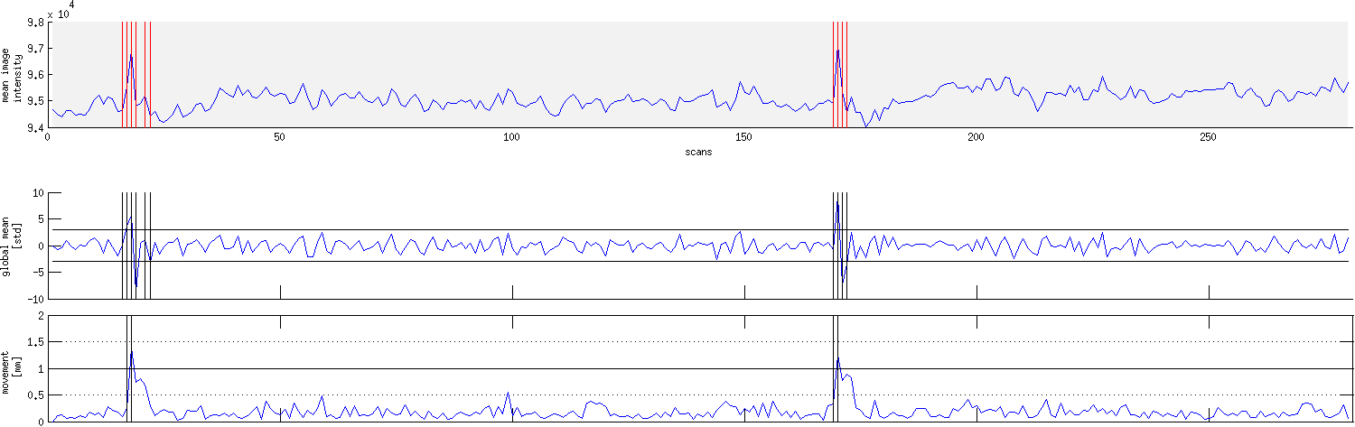
Almost no subjects lie perfectly still. As we can see from the sharp spikes in the graphs below, some move quite drastically. Severe, sudden movement can contaminate your analysis quite severely.

Motion correction tries to correct for smaller movements, but sometimes it’s best to just remove the images acquired during extreme rapid movement. We use Artifact Detection to identify the timepoints/images of the functional image that vary so much they should be excluded from further analysis and to label them so they are excluded from subsequent analyses.
For example, checking the translation and rotation graphs for a session shown above for sudden movement greater than 2 standard deviations from the mean, or for movement greater than 1mm, artifact detection would show that images 16-19, 21, 22 and 169-172 should be excluded from further analysis. The graph produced by artifact detection, with vertical lines corresponding to images with drastic variation is shown below.
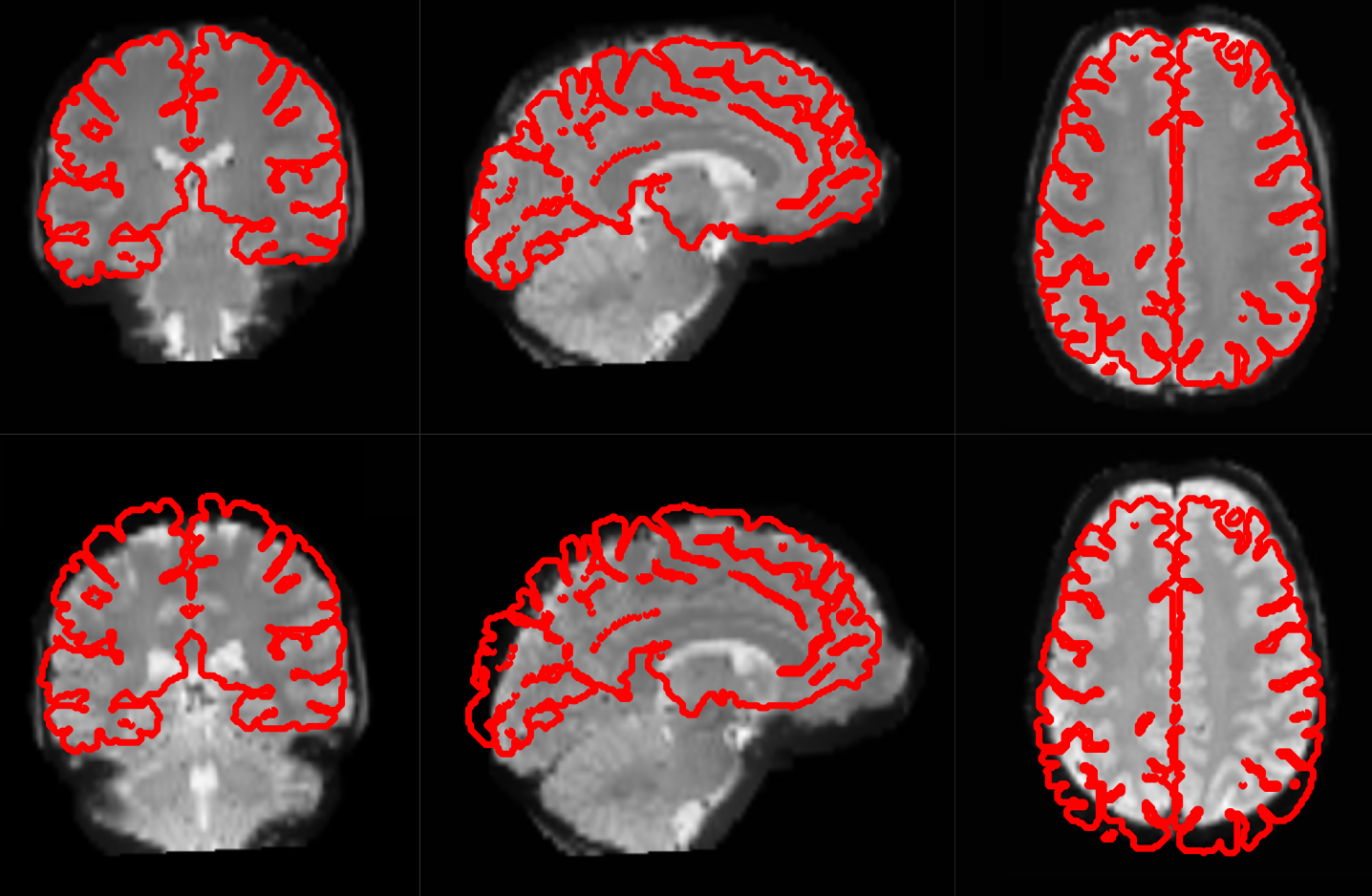
Motion correction aligns all the images within a volume so they are ‘aligned’. Coregistration aligns the functional image with the reference structural image. If you think of the functional image as having been printed on tracing paper, coregistration moves that image around on the reference image until the alignment is at its best. In other words, coregistration tries to superimpose the functional image perfectly on the anatomical image. This allows further transformations of the anatomical image, such as normalization, to be directly applied to the functional image.
The following picture shows an example of good (top) and bad (bottom) coregistration of functional images with the corresponding anatomical images. The red lines are the outline of the cortical folds of the anatomical image superimposed on the underlying greyscale functional image.
Every person’s brain is slightly different from every other’s. Brains differ in size and shape. To compare the images of one person’s brain to another’s, the images must first be translated onto a common shape and size, which is called normalization. Normalization maps data from the individual subject-space it was measured in onto a reference-space. Once this step is completed, a group analysis or comparison among data can be performed. There are different ways to normalize data but it always includes a template and a source image.
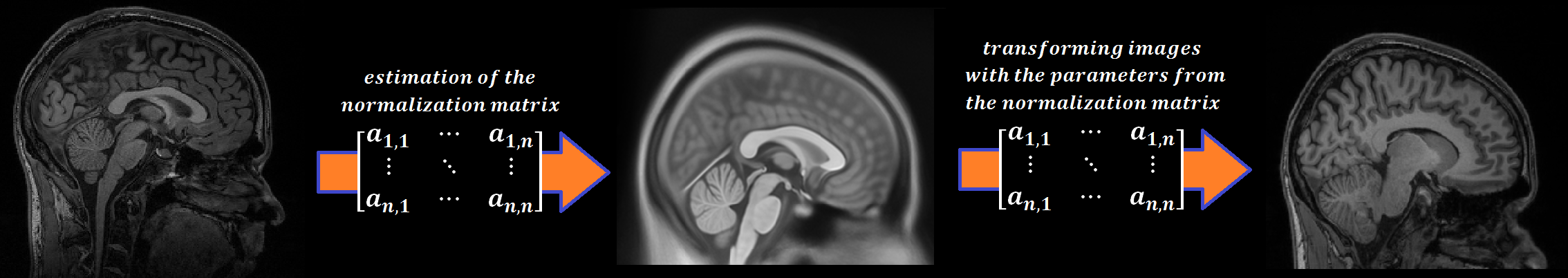
The template image is the standard brain in reference-space onto which you want to map your data. This can be a Talairach-, MNI-, or SPM-template, or some other reference image you choose to use.
The source image (normally a higher resolution structural image) is used to calculate the transformation matrix necessary to map the source image onto the template image. This transformation matrix is then used to map the rest of your images (functional and structural) into the reference-space.
Structural as well as functional images are smoothed by applying a filter to the image. Smoothing increases the signal to noise ratio of your data by filtering the highest frequencies from the frequency domain; that is, removing the smallest scale changes among voxels. That helps to make the larger scale changes more apparent. There is some inherent variability in functional location among individuals, and smoothing helps to reduce spatial differences between subjects and therefore aids comparing multiple subjects. The trade-off, of course, is that you lose resolution by smoothing. Keep in mind, though, that smoothing can cause regions that are functionally different to combine with each other. In such cases a surface based analysis with smoothing on the surface might be a better choice.
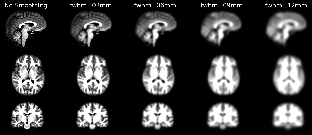
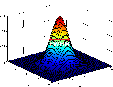
Smoothing is implemented by applying a 3D Gaussian kernel to the image, and the amount of smoothing is typically determined by its full width at half maximum (FWHM) parameter. As the name implies, FWHM is the width/diameter of the smoothing kernel at half of its height. Each voxel’s value is changed to the result of applying this smoothing kernel to its original value.
Choosing the size of the smoothing kernel also depends on your reason for smoothing. If you want to study a small region, a large kernel might smooth your data too much. The filter shouldn’t generally be larger than the activation you’re trying to detect. Thus, the amount of smoothing that you should use is determined partly by the question you want to answer. Some authors suggest using twice the voxel dimensions as a reasonable starting point.

Segmentation is the process by which a brain is divided into neurological sections according to a given template specification. This can be rather general, for example, segmenting the brain into gray matter, white matter and cerebrospinal fluid, as is done with SPM’s Segmentation, or quite detailed, segmenting into specific functional regions and their subregions, as is done with FreeSurfer’s recon-all, and that is illustrated in the figure.
Segmentation can be used for different things. You can use the segmentation to aid the normalization process or use it to aid further analysis by using a specific segmentation as a mask or as the definition of a specific region of interest (ROI).
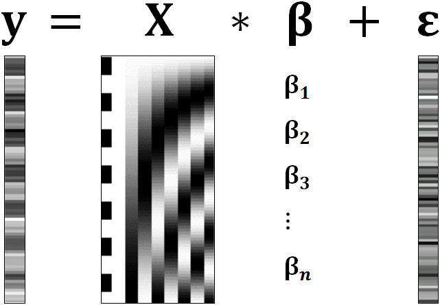
To test our hypothesis on our data we first need to specify a model that incorporates this hypothesis and accounts for multiple factors such as the expected function of the BOLD signal, the movement during measurement, experiment specify parameters and other regressors and covariates. Such a model is usually represented by a Generalized Linear Model (GLM).
A GLM describes a response (y), such as the BOLD response in a voxel, in terms of all its contributing factors (xβ) in a linear combination, whilst also accounting for the contribution of error (ε). The column (y) corresponds to one voxel and one row in this column corresponds to one time-point.
observed data (e.g. BOLD response in a single voxel)
e.g. experimental conditions (embodies all available knowledge about experimentally controlled factors and potential confounds), stimulus information (onset and duration of stimuli), expected shape of BOLD response
Quantifies how much each predictor (X) independently influences the dependent variable (Y)
Variance in the data (Y) which is not explained by the linear combination of predictors (Xβ). The error is assumed to be normally distributed.
The predictor variables are stored in a so called Design Matrix. The β parameters define the contribution of each component of this design matrix to the model. They are estimated so as to minimize the error, and are used to generate the contrasts between conditions. The Errors is the difference between the observed data and the model defined by Xβ.
BOLD responses have a delayed and dispersed form
We have to take the time delay and the HRF shape of the BOLD response into account when we create our design matrix.
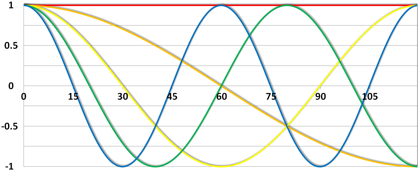
BOLD signals include substantial amounts of low-frequency noise
By high pass filtering our data and adding time regressors of 1st, 2nd,… order we can correct for low-frequency drifts in our measured data. This low frequency signals are caused by non-experimental effects, such as scanner drift etc.

This High pass Filter is established by setting up discrete cosine functions over the time period of your acquisition. In the example below you see a constant term of 1, followed by half of a cosine function increasing by half a period for each following curve. Such regressors correct for the influence of changes in the low-frequency spectrum.
Let us assume we have an experiment where we present subjects faces of humans and animals alike. Our goal is to measure the difference between the brain activation when a face of an animal is presented in contrast to the activation of the brain when a human face is presented. Our experiment is set up in such a way that subjects have two different blocks of stimuli presentation. In both blocks there are timepoints where faces of humans, faces of animals and no faces (resting state) are presented.
Now, we combine all that we know about our model into one single Design Matrix. This Matrix contains multiple columns, which contain information about the stimuli (onset, duration and curve function of the BOLD-signal i.e. the shape of the HRF). In our example column Sn(1) humans and Sn(1) animals code for the stimuli of humans and animals during the first session of our fictive experiment. Accordingly, Sn(2) codes for all the regressors in the second session. Sn(1) resting codes for the timepoints where subjects weren’t presented any stimuli.

The y-axis codes for the measured scan or the passed time, depending on the specification of your design. The x-axis stands for all the regressors that we specified.
The regressors Sn(1) R1 to Sn(1) R6 stand for the movement parameters we got from the realignment process. The regressors Sn(1) linear, Sn(1) quadratic, Sn(1) cubic and Sn(1) quartic are just examples of correction for the low frequency in your data. If you are using a high-pass filter of e.g. 128 seconds you don’t need to specifically include those regressors in your design matrix.
Note
Adding one more regressors to your model decrease the degrees of freedom in your statistical tests by one.
After we specified the parameters of our model in a design matrix we are ready to estimate our model. This means that we apply our model on the time course of each and every voxel.
Depending on the software you are using you might get different types of results. If you are using SPM the following images are created each time an analysis is performed (1st or 2nd level):
images of estimated regression coefficients (parameter estimate). beta images contain information about the size of the effect of interest. A given voxel in each beta image will have a value related to the size of effect for that explanatory variable.
ResMS-imageresidual sum of squares or variance image. It is a measure of within-subject error at the 1st level or between-subject error at the 2nd level analysis. This image is used to produce spmT images.
con-imagesduring contrast estimation beta images are linearly combined to produce relevant con-images
spmT-imagesduring contrast estimation the beta values of a con-image are combined with error values of the ResMS-image to calculate the t-value at each voxel
Before we go into the specifics of a statistical analysis, let me explain you the difference between a 1st and a 2nd level analysis.
A 1st level analysis is the statistical analysis done on each and every subject by itself. For this procedure the data doesn’t have to be normalized, i.e in a common reference space. A design matrix on this level controls for subject specific parameters as movement, respiration, heart beat, etc.
A 2nd level analysis is the statistical analysis done on the group. To be able to do this, our subject specific data has to be normalized and transformed from subject-space into reference-space. Otherwise we wouldn’t be able to compare subjects between each other. Additionally, all contrasts of the 1st level analysis have to be estimated because the model of the 2nd level analysis is conducted on them. The design matrix of the 2nd level analysis controls for subject specific parameters such as age, gender, socio-economic parameters, etc. At this point we also specify the group assignment of each subject.
Independent of the level of your analysis, after you’ve specified and estimated your model you now have to estimate the contrasts you are interested in. In such a contrast you specify how to weight the different regressors of your design matrix and combine them in one single image.
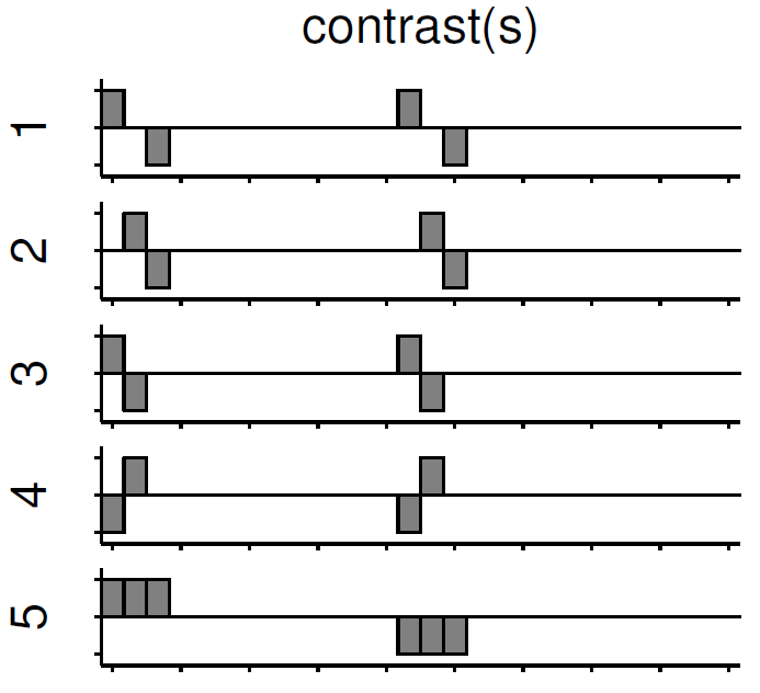
For example, if you want to compare the brain activation during the presentation of human faces compared to the brain activation during the presentation of animal faces over two sessions you have to weight the regressors Sn(1) humans and Sn(2) humans with 1 and Sn(1) animals and Sn(2) animals with -1, as can be seen in contrast 3. This will subtract the value of the animal-activation from the activation during the presentation of human faces. The result is an image where the positive activation stands for “more active” during the presentation of human faces than during the presentation of animal faces.
Contrast 1 codes for human faces vs. resting, contrast 2 codes for animal faces vs. resting, contrast 4 codes for animal faces vs. human faces (which is just the inverse image of contrast 3) and contrast 5 codes for session 1 vs. session 2, which looks for regions which were more active in the first session than in the second session.
After the contrasts are estimated there is only one final step to be taken before you get a scientific based answer to your question. You have to threshold your results. With that I mean, you have to specify the level of significance you want to test your data on, you have to correct for multiple comparison and you have to specify the parameters of the results you are looking for. E.g.:
FWE-correction: The family-wise error correction is one way to correct for multiple comparisons
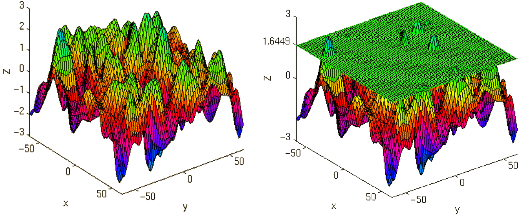
p-value: specify the hight of the significance threshold that you want to use (e.g. z=1.6449 equals p<0.05 (one-tailed); see image)
voxel extend: specify the minimum size of a “significant” cluster by specifying the number of voxel it at least has to contain.
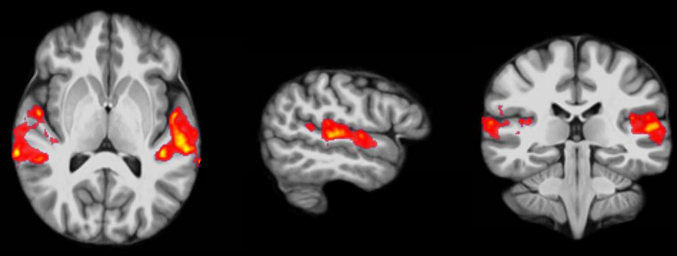
If you do all this correctly, you’ll end up with something as shown in the following picture. The picture shows you the average brain activation of 20 subjects during the presentation of an acoustic stimuli. The p-value are shown from red to yellow, representing values from 0.05 to 0.00. Shown are only cluster with a voxel extend of at least 100 voxels.