![]()
![]()
Important
This guide hasn’t been updated since January 2017 and is based on an older version of Nipype. The code in this guide is not tested against newer Nipype versions and might not work anymore. For a newer, more up to date and better introduction to Nipype, please check out the the Nipype Tutorial.
In this section you will learn how to create a workflow that does a second level analysis on fMRI data. There are again multiple ways how you can do this, but the most simple on is to check if your contrasts from the first level analysis are still significant on the group-level a.k.a. the 2nd level.
Note
You can only do a second level analysis if you already have done a first level analysis, obviously! But more importantly, those first level contrasts have to be in a common reference space. Otherwise there is now way of actually comparing them with each other and getting a valid results from them. Luckily, if you’ve done the previous step, you’ve already normalized your data (either with ANTs or SPM) to a template.
If you’ve already done the previous sections, you know how this works. We first import necessary modules, define experiment specific parameters, create nodes, create a workflow and connect the nodes to it, we create an I/O stream and connect it to the workflow and finally run this workflow.
1 2 3 4 5 6 7 8 9 10 11 | from os.path import join as opj
from nipype.interfaces.io import SelectFiles, DataSink
from nipype.interfaces.spm import (OneSampleTTestDesign, EstimateModel,
EstimateContrast, Threshold)
from nipype.interfaces.utility import IdentityInterface
from nipype.pipeline.engine import Workflow, Node
# Specification to MATLAB
from nipype.interfaces.matlab import MatlabCommand
MatlabCommand.set_default_paths('/usr/local/MATLAB/R2014a/toolbox/spm12')
MatlabCommand.set_default_matlab_cmd("matlab -nodesktop -nosplash")
|
1 2 3 4 5 6 7 8 9 10 | experiment_dir = '~/nipype_tutorial' # location of experiment folder
output_dir = 'output_fMRI_example_2nd_ants' # name of 2nd-level output folder
input_dir_norm = 'output_fMRI_example_norm_ants'# name of norm output folder
working_dir = 'workingdir_fMRI_example_2nd_ants'# name of working directory
subject_list = ['sub001', 'sub002', 'sub003',
'sub004', 'sub005', 'sub006',
'sub007', 'sub008', 'sub009',
'sub010'] # list of subject identifiers
contrast_list = ['con_0001', 'con_0002', 'con_0003',
'con_0004', 'ess_0005', 'ess_0006'] # list of contrast identifiers
|
Note
Pay attention to the name of the input_dir_norm. Depending on the way you normalized your data, ANTs or SPM, the folder name has either the ending _ants or _spm.
We don’t need many nodes for a simple second level analysis. In fact they are the same as the ones we used for the first level analysis. We create a simple T-Test, estimate it and look at a simple mean contrast, i.e. a contrast that shows what the group mean activation of a certain first level contrast is.
1 2 3 4 5 6 7 8 9 10 11 12 13 | # One Sample T-Test Design - creates one sample T-Test Design
onesamplettestdes = Node(OneSampleTTestDesign(),
name="onesampttestdes")
# EstimateModel - estimate the parameters of the model
level2estimate = Node(EstimateModel(estimation_method={'Classical': 1}),
name="level2estimate")
# EstimateContrast - estimates simple group contrast
level2conestimate = Node(EstimateContrast(group_contrast=True),
name="level2conestimate")
cont1 = ['Group', 'T', ['mean'], [1]]
level2conestimate.inputs.contrasts = [cont1]
|
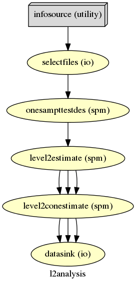
1 2 3 4 5 6 7 8 9 10 11 12 13 14 | # Specify 2nd-Level Analysis Workflow & Connect Nodes
l2analysis = Workflow(name='l2analysis')
l2analysis.base_dir = opj(experiment_dir, working_dir)
# Connect up the 2nd-level analysis components
l2analysis.connect([(onesamplettestdes, level2estimate, [('spm_mat_file',
'spm_mat_file')] ),
(level2estimate, level2conestimate, [('spm_mat_file',
'spm_mat_file'),
('beta_images',
'beta_images'),
('residual_image',
'residual_image')]),
])
|
The creation of the I/O stream is as usual. But because I showed you three ways to normalize your data in the previous section, be aware that you have to point the SelectFiles node to the right input folder. Your option for the SelectFiles input template are as follows:
1 2 3 4 5 6 7 8 9 10 11 | # contrast template for ANTs normalization (complete)
con_file = opj(input_dir_norm, 'warp_complete', 'sub*', 'warpall*',
'{contrast_id}_trans.nii')
# contrast template for ANTs normalization (partial)
con_file = opj(input_dir_norm, 'warp_partial', 'sub*', 'apply2con*',
'{contrast_id}_out_trans.nii.gz')
# contrast template for SPM normalization
con_file = opj(input_dir_norm, 'normalized', 'sub*',
'*{contrast_id}_out.nii')
|
Note
It is very important to notice that only contrast images (e.g. con-images) can be used for a second-level group analysis. It is statistically incorrect to use statistic images, such as spmT- or spmF-images.
The following example is adjusted for the situation where the normalization was done with ANTs. The code for the I/O stream looks as follows:
1 2 3 4 5 6 7 8 9 10 11 12 13 14 15 16 17 18 19 20 21 22 23 24 25 26 27 28 29 30 31 32 33 34 | # Infosource - a function free node to iterate over the list of subject names
infosource = Node(IdentityInterface(fields=['contrast_id']),
name="infosource")
infosource.iterables = [('contrast_id', contrast_list)]
# SelectFiles - to grab the data (alternative to DataGrabber)
con_file = opj(input_dir_norm, 'warp_complete', 'sub*', 'warpall*',
'{contrast_id}_trans.nii')
templates = {'cons': con_file}
selectfiles = Node(SelectFiles(templates,
base_directory=experiment_dir),
name="selectfiles")
# Datasink - creates output folder for important outputs
datasink = Node(DataSink(base_directory=experiment_dir,
container=output_dir),
name="datasink")
# Use the following DataSink output substitutions
substitutions = [('_contrast_id_', '')]
datasink.inputs.substitutions = substitutions
# Connect SelectFiles and DataSink to the workflow
l2analysis.connect([(infosource, selectfiles, [('contrast_id',
'contrast_id')]),
(selectfiles, onesamplettestdes, [('cons', 'in_files')]),
(level2conestimate, datasink, [('spm_mat_file',
'contrasts.@spm_mat'),
('spmT_images',
'contrasts.@T'),
('con_images',
'contrasts.@con')]),
])
|
If you’ve normalized your data with ANTs but did only the so called partial approach, the code above will not work and crash with the following message:
1 2 3 4 5 6 7 8 | Item 'Scans', field 'val': Number of matching files (0) less than required (1).
Standard error:
MATLAB code threw an exception:
...
Name:pyscript_onesamplettestdesign
...
Interface OneSampleTTestDesign failed to run.
|
Such errors are sometimes hard to read. What this message means is that SPM’s onesamplettestdes tried to open an image-file but was only able to read out 0 scans, of the requested at least 1. This is a common message where SPM tries to read a zipped NIfTI file (ending with nii.gz) and cannot unpack it. To solve this issue we only need to insert an additional Gunzip node in our pipeline and redirect the workflow through this new gunzip node before it goes to the onesamplettestdes node. So the new code looks as follows:
1 2 3 4 5 6 7 8 9 10 11 12 13 14 15 16 17 18 19 | # Gunzip - unzip the contrast image
from nipype.algorithms.misc import Gunzip
from nipype.pipeline.engine import MapNode
gunzip_con = MapNode(Gunzip(), name="gunzip_con",
iterfield=['in_file'])
# Connect SelectFiles and DataSink to the workflow
l2analysis.connect([(infosource, selectfiles, [('contrast_id',
'contrast_id')]),
(selectfiles, gunzip_con, [('cons', 'in_file')]),
(gunzip_con, onesamplettestdes, [('out_file',
'in_files')]),
(level2conestimate, datasink, [('spm_mat_file',
'contrasts.@spm_mat'),
('spmT_images',
'contrasts.@T'),
('con_images',
'contrasts.@con')]),
])
|
1 2 | l2analysis.write_graph(graph2use='colored')
l2analysis.run('MultiProc', plugin_args={'n_procs': 8})
|
Hint
You can download the code for this 2nd level pipeline as a script here: example_fMRI_3_second_level.py
The resulting folder structure looks as follows:
output_fMRI_example_2nd
|-- contrasts
    |-- con_0001
    |   |-- con_0001.nii
    |   |-- SPM.mat
    |   |-- spmT_0001.nii
    |-- con_0002
    |-- con_0003
    |-- con_0004
    |-- ess_0005
    |   |-- ess_0005.nii
    |   |-- SPM.mat
    |   |-- spmF_0005.nii
    |-- ess_0006